

82
3 Modeling Composite Structures
3.10 Computing a Green’s Function for a Layered
Workpiece
We now consider a layered workpiece of finite extent in the z-direction. We assume
that the source is at z > 0, the workpiece has a thickness, z w , satisfies −z w < z <
0, and is divided into, say, ten subregions, which are defined as follows:
Layer1 :
z 1 < z < z 0 = 0
Layer2 :
z 2 < z < z 1
. . .
. . .
Layer10 : −z w = z 10 < z < z 9
.
(3.20)
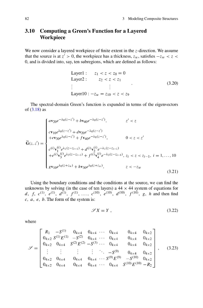
The spectral-domain Green’s function is expanded in terms of the eigenvectors
of (3.18) as
G(z, z ) =
⎧
⎪ ⎪ ⎪ ⎪ ⎪ ⎪ ⎪ ⎪ ⎪ ⎪ ⎪ ⎪ ⎪ ⎪ ⎨
⎪ ⎪ ⎪ ⎪ ⎪ ⎪ ⎪ ⎪ ⎪ ⎪ ⎪ ⎪ ⎪ ⎪ ⎩
av 20 e −λ 0 (z−z ) + bv 40 e −λ 0 (z−z ) ,
z < z
cv 10 e λ 0 (z−z ) + dv 20 e −λ 0 (z−z )
+ev 30 e λ 0 (z−z ) + f v 40 e −λ 0 (z−z ) ,
0 < z < z
c (i) v
(i)
1 e λ 1 (z−z i−1 ) + d (i) v
(i)
2 e −λ 1 (z−z i−1 )
+e (i) v
(i)
3 e λ 3 (z−z i−1 ) + f (i) v
(i)
4 e −λ 3 (z−z i−1 ) , z i < z < z i−1 , i = 1, . . . , 10
gv 10 e λ 0 (z+z w ) + hv 30 e λ 0 (z+z w ) ,
z< −z w
(3.21)
Using the boundary conditions and the conditions at the source, we can find the
unknowns by solving (in the case of ten layers) a 44 × 44 system of equations for
d, f, c (1) , e (1) , d (1) , f (1) , . . . , c (10) , e (10) , d (10) , f (10) , g, h and then find
c, a, e, b. The form of the system is:
S X = Y ,
(3.22)
where
S =
⎡
⎢
⎢
⎢
⎢
⎢
⎢
⎢
⎢
⎣
R 1 −S (1)
0 4×4 0 4×4 · · · 0 4×4
0 4×4 0 4×2
0 4×2 S (1) E (1) −S (2) 0 4×4 · · · 0 4×4
0 4×4 0 4×2
0 4×2 0 4×4 S (2) E (2) −S (3) · · · 0 4×4
0 4×4 0 4×2
. . .
. . .
. . .
. . .
. . . −S (9)
0 4×4 0 4×2
0 4×2 0 4×4
0 4×4 0 4×4 · · · S (9) E (9) −S (10) 0 4×2
0 4×2 0 4×4
0 4×4 0 4×4 · · · 0 4×4 S (10) E (10) −R 2
⎤
⎥
⎥
⎥
⎥
⎥
⎥
⎥
⎥
⎦
,
(3.23)
3 Modeling Composite Structures
3.10 Computing a Green’s Function for a Layered
Workpiece
We now consider a layered workpiece of finite extent in the z-direction. We assume
that the source is at z > 0, the workpiece has a thickness, z w , satisfies −z w < z <
0, and is divided into, say, ten subregions, which are defined as follows:
Layer1 :
z 1 < z < z 0 = 0
Layer2 :
z 2 < z < z 1
. . .
. . .
Layer10 : −z w = z 10 < z < z 9
.
(3.20)
The spectral-domain Green’s function is expanded in terms of the eigenvectors
of (3.18) as
G(z, z ) =
⎧
⎪ ⎪ ⎪ ⎪ ⎪ ⎪ ⎪ ⎪ ⎪ ⎪ ⎪ ⎪ ⎪ ⎪ ⎨
⎪ ⎪ ⎪ ⎪ ⎪ ⎪ ⎪ ⎪ ⎪ ⎪ ⎪ ⎪ ⎪ ⎪ ⎩
av 20 e −λ 0 (z−z ) + bv 40 e −λ 0 (z−z ) ,
z < z
cv 10 e λ 0 (z−z ) + dv 20 e −λ 0 (z−z )
+ev 30 e λ 0 (z−z ) + f v 40 e −λ 0 (z−z ) ,
0 < z < z
c (i) v
(i)
1 e λ 1 (z−z i−1 ) + d (i) v
(i)
2 e −λ 1 (z−z i−1 )
+e (i) v
(i)
3 e λ 3 (z−z i−1 ) + f (i) v
(i)
4 e −λ 3 (z−z i−1 ) , z i < z < z i−1 , i = 1, . . . , 10
gv 10 e λ 0 (z+z w ) + hv 30 e λ 0 (z+z w ) ,
z< −z w
(3.21)
Using the boundary conditions and the conditions at the source, we can find the
unknowns by solving (in the case of ten layers) a 44 × 44 system of equations for
d, f, c (1) , e (1) , d (1) , f (1) , . . . , c (10) , e (10) , d (10) , f (10) , g, h and then find
c, a, e, b. The form of the system is:
S X = Y ,
(3.22)
where
S =
⎡
⎢
⎢
⎢
⎢
⎢
⎢
⎢
⎢
⎣
R 1 −S (1)
0 4×4 0 4×4 · · · 0 4×4
0 4×4 0 4×2
0 4×2 S (1) E (1) −S (2) 0 4×4 · · · 0 4×4
0 4×4 0 4×2
0 4×2 0 4×4 S (2) E (2) −S (3) · · · 0 4×4
0 4×4 0 4×2
. . .
. . .
. . .
. . .
. . . −S (9)
0 4×4 0 4×2
0 4×2 0 4×4
0 4×4 0 4×4 · · · S (9) E (9) −S (10) 0 4×2
0 4×2 0 4×4
0 4×4 0 4×4 · · · 0 4×4 S (10) E (10) −R 2
⎤
⎥
⎥
⎥
⎥
⎥
⎥
⎥
⎥
⎦
,
(3.23)