

80
3 Modeling Composite Structures
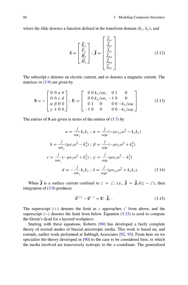
where the tilde denotes a function defined in the transform domain (k x , k y ), and
e =
⎡
⎢
⎢
⎣
E x
E y
H x
H y
⎤
⎥
⎥
⎦ ; J =
⎡
⎢
⎢
⎢
⎢
⎢
⎢
⎢
⎣
J ex
J ey
J ez
J mx
J my
J mz
⎤
⎥
⎥
⎥
⎥
⎥
⎥
⎥
⎦
.
(3.12)
The subscript e denotes an electric current, and m denotes a magnetic current. The
matrices in (3.9) are given by
S = −
⎡
⎢
⎢
⎣
0 0 a b
0 0 c d
α β 0 0
γ δ 0 0
⎤
⎥
⎥
⎦ ; U =
⎡
⎢
⎢
⎣
0 0 k x /ωω z 0 1
0
0 0 k y /ωω z −1 0
0
0 1
0
0 0 −k x /ωμ
−1 0
0
0 0 −k y /ωμ
⎤
⎥
⎥
⎦ .
(3.13)
The entries of S are given in terms of the entries of (3.7) by
a =
j
ωω z
k x k y ; α =
j
ωμ
(−μμ yx ω
2
− k x k y )
b =
j
ωω z
(μμ z ω
2
− k
2
x ) ; β =
j
ωμ
(−μμ y ω
2
+ k
2
x )
c =
j
ωω z
(−μμ z ω
2
+ k
2
y ) ; γ =
j
ωμ
(μμ x ω
2
− k
2
y )
d = −
j
ωω z
k x k y ; δ =
j
ωμ
(μμ xy ω
2
+ k x k y ).
(3.14)
When J is a surface current confined to z = z , i.e., J = J s δ(z − z ), then
integration of (3.9) produces
e
(+)
− e
(−)
= U · J s .
(3.15)
The superscript (+) denotes the limit as z approaches z from above, and the
superscript (−) denotes the limit from below. Equation (3.15) is used to compute
the Green’s dyad for a layered workpiece.
Starting with these equations, Roberts [90] has developed a fairly complete
theory of normal modes of biaxial anisotropic media. This work is based on, and
extends, earlier work performed at Sabbagh Associates [92, 93]. From here on we
specialize the theory developed in [90] to the case to be considered here, in which
the media involved are transversely isotropic to the x-coordinate. The generalized
3 Modeling Composite Structures
where the tilde denotes a function defined in the transform domain (k x , k y ), and
e =
⎡
⎢
⎢
⎣
E x
E y
H x
H y
⎤
⎥
⎥
⎦ ; J =
⎡
⎢
⎢
⎢
⎢
⎢
⎢
⎢
⎣
J ex
J ey
J ez
J mx
J my
J mz
⎤
⎥
⎥
⎥
⎥
⎥
⎥
⎥
⎦
.
(3.12)
The subscript e denotes an electric current, and m denotes a magnetic current. The
matrices in (3.9) are given by
S = −
⎡
⎢
⎢
⎣
0 0 a b
0 0 c d
α β 0 0
γ δ 0 0
⎤
⎥
⎥
⎦ ; U =
⎡
⎢
⎢
⎣
0 0 k x /ωω z 0 1
0
0 0 k y /ωω z −1 0
0
0 1
0
0 0 −k x /ωμ
−1 0
0
0 0 −k y /ωμ
⎤
⎥
⎥
⎦ .
(3.13)
The entries of S are given in terms of the entries of (3.7) by
a =
j
ωω z
k x k y ; α =
j
ωμ
(−μμ yx ω
2
− k x k y )
b =
j
ωω z
(μμ z ω
2
− k
2
x ) ; β =
j
ωμ
(−μμ y ω
2
+ k
2
x )
c =
j
ωω z
(−μμ z ω
2
+ k
2
y ) ; γ =
j
ωμ
(μμ x ω
2
− k
2
y )
d = −
j
ωω z
k x k y ; δ =
j
ωμ
(μμ xy ω
2
+ k x k y ).
(3.14)
When J is a surface current confined to z = z , i.e., J = J s δ(z − z ), then
integration of (3.9) produces
e
(+)
− e
(−)
= U · J s .
(3.15)
The superscript (+) denotes the limit as z approaches z from above, and the
superscript (−) denotes the limit from below. Equation (3.15) is used to compute
the Green’s dyad for a layered workpiece.
Starting with these equations, Roberts [90] has developed a fairly complete
theory of normal modes of biaxial anisotropic media. This work is based on, and
extends, earlier work performed at Sabbagh Associates [92, 93]. From here on we
specialize the theory developed in [90] to the case to be considered here, in which
the media involved are transversely isotropic to the x-coordinate. The generalized