

36
2 Voxel-Based Inversion Via Set-Theoretic Estimation
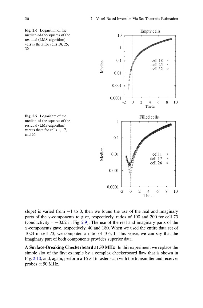
Fig. 2.6 Logarithm of the
median-of-the-squares of the
residual (LMS-algorithm)
versus theta for cells 18, 25,
32
0.0001
0.001
0.01
0.1
1
10
-2 0
2
4
6
8 10
Median
Theta
Empty cells
cell 18
cell 25
cell 32
Fig. 2.7 Logarithm of the
median-of-the-squares of the
residual (LMS-algorithm)
versus theta for cells 1, 17,
and 26
0.0001
0.001
0.01
0.1
1
-2 0
2
4
6
8 10
Median
Theta
Filled cells
cell 1
cell 17
cell 26
slope) is varied from −1 to 0, then we found the use of the real and imaginary
parts of the y-components to give, respectively, ratios of 100 and 200 for cell 73
(conductivity = −0.02 in Fig. 2.9). The use of the real and imaginary parts of the
x-components gave, respectively, 40 and 180. When we used the entire data set of
1024 in cell 73, we computed a ratio of 105. In this sense, we can say that the
imaginary part of both components provides superior data.
A Surface-Breaking Checkerboard at 50 MHz In this experiment we replace the
simple slot of the first example by a complex checkerboard flaw that is shown in
Fig. 2.10, and, again, perform a 16 × 16 raster scan with the transmitter and receiver
probes at 50 MHz.
2 Voxel-Based Inversion Via Set-Theoretic Estimation
Fig. 2.6 Logarithm of the
median-of-the-squares of the
residual (LMS-algorithm)
versus theta for cells 18, 25,
32
0.0001
0.001
0.01
0.1
1
10
-2 0
2
4
6
8 10
Median
Theta
Empty cells
cell 18
cell 25
cell 32
Fig. 2.7 Logarithm of the
median-of-the-squares of the
residual (LMS-algorithm)
versus theta for cells 1, 17,
and 26
0.0001
0.001
0.01
0.1
1
-2 0
2
4
6
8 10
Median
Theta
Filled cells
cell 1
cell 17
cell 26
slope) is varied from −1 to 0, then we found the use of the real and imaginary
parts of the y-components to give, respectively, ratios of 100 and 200 for cell 73
(conductivity = −0.02 in Fig. 2.9). The use of the real and imaginary parts of the
x-components gave, respectively, 40 and 180. When we used the entire data set of
1024 in cell 73, we computed a ratio of 105. In this sense, we can say that the
imaginary part of both components provides superior data.
A Surface-Breaking Checkerboard at 50 MHz In this experiment we replace the
simple slot of the first example by a complex checkerboard flaw that is shown in
Fig. 2.10, and, again, perform a 16 × 16 raster scan with the transmitter and receiver
probes at 50 MHz.