

2.5 Some Examples of the Inversion Algorithm
35
8
9 10 11 12
15
17
20
27 28
32
34 35
39
45
1
2
3
4
5
6
7
13 14
29
22
36
43
16
23
30
37
44
24
31
38
18
25
46
19
26
33
40
47
41
48
21
42
49
y
x
Cell Numbers
-0.4
-0.3
-0.2
-0.1
0
0.1
0.2
0.3
0.4
-1 -0.5 0
0.5
1
1.5
J (Amp/m**2)
E (Volts/m)
J versus E: Cell 1
real x
imag x
real y
imag y
-1
-0.8
-0.6
-0.4
-0.2
0
0.2
0.4
0.6
0.8
-1.5 -1 -0.5 0 0.5 1 1.5
J (Amp/m**2)
E (Volts/m)
J versus E: Cell 17
real x
imag x
real y
imag y
-1
-0.8
-0.6
-0.4
-0.2
0
0.2
0.4
0.6
0.8
1
-1.5 -1 -0.5 0 0.5 1 1.5
J (Amp/m**2)
E (Volts/m)
J versus E: Cell 26
real x
imag x
real y
imag y
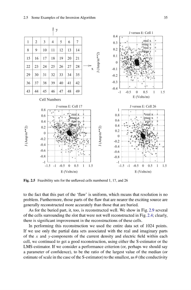
Fig. 2.5 Feasibility sets for the unflawed cells numbered 1, 17, and 26
to the fact that this part of the ‘flaw’ is uniform, which means that resolution is no
problem. Furthermore, those parts of the flaw that are nearer the exciting source are
generally reconstructed more accurately than those that are buried.
As for the buried part, it, too, is reconstructed well. We show in Fig. 2.9 several
of the cells surrounding the slot that were not well reconstructed in Fig. 2.4; clearly,
there is significant improvement in the reconstructions of these cells.
In performing this reconstruction we used the entire data set of 1024 points.
If we use only the partial data sets associated with the real and imaginary parts
of the x and y-components of the current density and electric field within each
cell, we continued to get a good reconstruction, using either the S-estimator or the
LMS-estimator. If we consider a performance criterion (or, perhaps we should say
a parameter of confidence), to be the ratio of the largest value of the median (or
estimate of scale in the case of the S-estimator) to the smallest, as θ (the conductivity
35
8
9 10 11 12
15
17
20
27 28
32
34 35
39
45
1
2
3
4
5
6
7
13 14
29
22
36
43
16
23
30
37
44
24
31
38
18
25
46
19
26
33
40
47
41
48
21
42
49
y
x
Cell Numbers
-0.4
-0.3
-0.2
-0.1
0
0.1
0.2
0.3
0.4
-1 -0.5 0
0.5
1
1.5
J (Amp/m**2)
E (Volts/m)
J versus E: Cell 1
real x
imag x
real y
imag y
-1
-0.8
-0.6
-0.4
-0.2
0
0.2
0.4
0.6
0.8
-1.5 -1 -0.5 0 0.5 1 1.5
J (Amp/m**2)
E (Volts/m)
J versus E: Cell 17
real x
imag x
real y
imag y
-1
-0.8
-0.6
-0.4
-0.2
0
0.2
0.4
0.6
0.8
1
-1.5 -1 -0.5 0 0.5 1 1.5
J (Amp/m**2)
E (Volts/m)
J versus E: Cell 26
real x
imag x
real y
imag y
Fig. 2.5 Feasibility sets for the unflawed cells numbered 1, 17, and 26
to the fact that this part of the ‘flaw’ is uniform, which means that resolution is no
problem. Furthermore, those parts of the flaw that are nearer the exciting source are
generally reconstructed more accurately than those that are buried.
As for the buried part, it, too, is reconstructed well. We show in Fig. 2.9 several
of the cells surrounding the slot that were not well reconstructed in Fig. 2.4; clearly,
there is significant improvement in the reconstructions of these cells.
In performing this reconstruction we used the entire data set of 1024 points.
If we use only the partial data sets associated with the real and imaginary parts
of the x and y-components of the current density and electric field within each
cell, we continued to get a good reconstruction, using either the S-estimator or the
LMS-estimator. If we consider a performance criterion (or, perhaps we should say
a parameter of confidence), to be the ratio of the largest value of the median (or
estimate of scale in the case of the S-estimator) to the smallest, as θ (the conductivity