

34
2 Voxel-Based Inversion Via Set-Theoretic Estimation
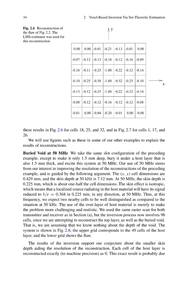
Fig. 2.4 Reconstruction of
the flaw of Fig. 2.2. The
LMS-estimator was used for
this reconstruction
-0.01
-0.16 -0.09
-0.22
-0.25 -0.30
-0.32 -0.25
-0.12
-1.00
-0.12 -0.16
-0.12 -0.08
-0.21 -0.13 -0.01
-0.07 -0.13 -0.13 -0.18 -0.12
-0.11 -0.25
-0.12 -0.14
-0.10
-0.16
-0.10
-0.13
-0.25
-0.22 -0.23 -0.14
-0.08 -0.12
-0.12
-0.01
-0.04 -0.20 -0.01
-1.00
0.00 0.00
0.00
-1.00
0.00
0.00 0.00
y
x
these results in Fig. 2.6 for cells 18, 25, and 32, and in Fig. 2.7 for cells 1, 17, and
26.
We will use figures such as these in some of our other examples to explain the
results of reconstructions.
Buried Void at 50 MHz We take the same slot configuration of the preceding
example, except to make it only 1.5 mm deep, bury it under a host layer that is
also 1.5 mm thick, and excite this system at 50 MHz. Our use of 50 MHz stems
from our interest in improving the resolution of the reconstructions of the preceding
example, and is guided by the following argument. The (x, y) cell dimensions are
0.429 mm, and the skin depth at 50 kHz is 7.12 mm. At 50 MHz, the skin depth is
0.225 mm, which is about one-half the cell dimensions. The skin effect is isotropic,
which means that a localized source radiating in the host material will have its signal
reduced to 1/e = 0.368 in 0.225 mm, in any direction, at 50 MHz. Thus, at this
frequency, we expect two nearby cells to be well distinguished as compared to the
situation at 50 kHz. The use of the over-layer of host material is merely to make
the problem more challenging and realistic. We used the same raster scan for both
transmitter and receiver as in Section (a), but the inversion process now involves 98
cells, since we are attempting to reconstruct the top layer, as well as the buried void.
That is, we are assuming that we know nothing about the depth of the void. The
system is shown in Fig. 2.8; the upper grid corresponds to the 49 cells of the host
layer, and the lower grid shows the flaw.
The results of the inversion support our conjecture about the smaller skin
depth aiding the resolution of the reconstruction. Each cell of the host layer is
reconstructed exactly (to machine precision) as 0. This exact result is probably due
2 Voxel-Based Inversion Via Set-Theoretic Estimation
Fig. 2.4 Reconstruction of
the flaw of Fig. 2.2. The
LMS-estimator was used for
this reconstruction
-0.01
-0.16 -0.09
-0.22
-0.25 -0.30
-0.32 -0.25
-0.12
-1.00
-0.12 -0.16
-0.12 -0.08
-0.21 -0.13 -0.01
-0.07 -0.13 -0.13 -0.18 -0.12
-0.11 -0.25
-0.12 -0.14
-0.10
-0.16
-0.10
-0.13
-0.25
-0.22 -0.23 -0.14
-0.08 -0.12
-0.12
-0.01
-0.04 -0.20 -0.01
-1.00
0.00 0.00
0.00
-1.00
0.00
0.00 0.00
y
x
these results in Fig. 2.6 for cells 18, 25, and 32, and in Fig. 2.7 for cells 1, 17, and
26.
We will use figures such as these in some of our other examples to explain the
results of reconstructions.
Buried Void at 50 MHz We take the same slot configuration of the preceding
example, except to make it only 1.5 mm deep, bury it under a host layer that is
also 1.5 mm thick, and excite this system at 50 MHz. Our use of 50 MHz stems
from our interest in improving the resolution of the reconstructions of the preceding
example, and is guided by the following argument. The (x, y) cell dimensions are
0.429 mm, and the skin depth at 50 kHz is 7.12 mm. At 50 MHz, the skin depth is
0.225 mm, which is about one-half the cell dimensions. The skin effect is isotropic,
which means that a localized source radiating in the host material will have its signal
reduced to 1/e = 0.368 in 0.225 mm, in any direction, at 50 MHz. Thus, at this
frequency, we expect two nearby cells to be well distinguished as compared to the
situation at 50 kHz. The use of the over-layer of host material is merely to make
the problem more challenging and realistic. We used the same raster scan for both
transmitter and receiver as in Section (a), but the inversion process now involves 98
cells, since we are attempting to reconstruct the top layer, as well as the buried void.
That is, we are assuming that we know nothing about the depth of the void. The
system is shown in Fig. 2.8; the upper grid corresponds to the 49 cells of the host
layer, and the lower grid shows the flaw.
The results of the inversion support our conjecture about the smaller skin
depth aiding the resolution of the reconstruction. Each cell of the host layer is
reconstructed exactly (to machine precision) as 0. This exact result is probably due