

2.5 Some Examples of the Inversion Algorithm
33
8
9 10 11 12
15
17
20
27 28
32
34 35
39
45
1
2
3
4
5
6
7
13 14
29
22
36
43
16
23
30
37
44
24
31
38
18
25
46
19
26
33
40
47
41
48
21
42
49
y
x
Cell Numbers
-4
-3
-2
-1
0
1
2
3
4
-4 -3 -2 -1 0 1 2 3
J (Amp/m**2)
E (Volts/m)
J versus E: Cell 18
real x
imag x
real y
imag y
-4
-3
-2
-1
0
1
2
3
4
-4 -3 -2 -1 0 1 2 3 4
J (Amp/m**2)
E (Volts/m)
J versus E: Cell 25
real x
imag x
real y
imag y
-4
-3
-2
-1
0
1
2
3
4
-3 -2 -1 0 1 2 3 4
J (Amp/m**2)
E (Volts/m)
J versus E: Cell 32
real x
imag x
real y
imag y
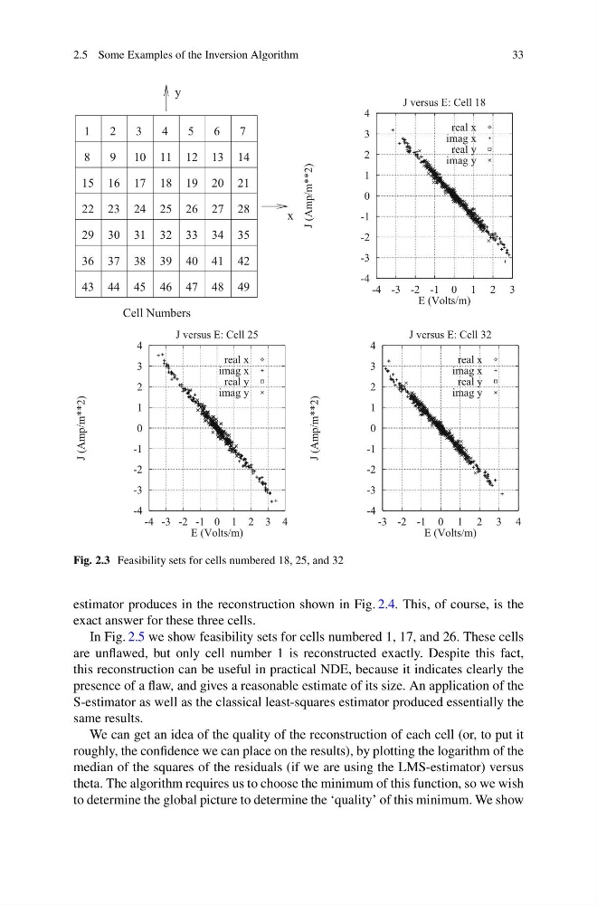
Fig. 2.3 Feasibility sets for cells numbered 18, 25, and 32
estimator produces in the reconstruction shown in Fig. 2.4. This, of course, is the
exact answer for these three cells.
In Fig. 2.5 we show feasibility sets for cells numbered 1, 17, and 26. These cells
are unflawed, but only cell number 1 is reconstructed exactly. Despite this fact,
this reconstruction can be useful in practical NDE, because it indicates clearly the
presence of a flaw, and gives a reasonable estimate of its size. An application of the
S-estimator as well as the classical least-squares estimator produced essentially the
same results.
We can get an idea of the quality of the reconstruction of each cell (or, to put it
roughly, the confidence we can place on the results), by plotting the logarithm of the
median of the squares of the residuals (if we are using the LMS-estimator) versus
theta. The algorithm requires us to choose the minimum of this function, so we wish
to determine the global picture to determine the ‘quality’ of this minimum. We show
33
8
9 10 11 12
15
17
20
27 28
32
34 35
39
45
1
2
3
4
5
6
7
13 14
29
22
36
43
16
23
30
37
44
24
31
38
18
25
46
19
26
33
40
47
41
48
21
42
49
y
x
Cell Numbers
-4
-3
-2
-1
0
1
2
3
4
-4 -3 -2 -1 0 1 2 3
J (Amp/m**2)
E (Volts/m)
J versus E: Cell 18
real x
imag x
real y
imag y
-4
-3
-2
-1
0
1
2
3
4
-4 -3 -2 -1 0 1 2 3 4
J (Amp/m**2)
E (Volts/m)
J versus E: Cell 25
real x
imag x
real y
imag y
-4
-3
-2
-1
0
1
2
3
4
-3 -2 -1 0 1 2 3 4
J (Amp/m**2)
E (Volts/m)
J versus E: Cell 32
real x
imag x
real y
imag y
Fig. 2.3 Feasibility sets for cells numbered 18, 25, and 32
estimator produces in the reconstruction shown in Fig. 2.4. This, of course, is the
exact answer for these three cells.
In Fig. 2.5 we show feasibility sets for cells numbered 1, 17, and 26. These cells
are unflawed, but only cell number 1 is reconstructed exactly. Despite this fact,
this reconstruction can be useful in practical NDE, because it indicates clearly the
presence of a flaw, and gives a reasonable estimate of its size. An application of the
S-estimator as well as the classical least-squares estimator produced essentially the
same results.
We can get an idea of the quality of the reconstruction of each cell (or, to put it
roughly, the confidence we can place on the results), by plotting the logarithm of the
median of the squares of the residuals (if we are using the LMS-estimator) versus
theta. The algorithm requires us to choose the minimum of this function, so we wish
to determine the global picture to determine the ‘quality’ of this minimum. We show