

32
2 Voxel-Based Inversion Via Set-Theoretic Estimation
3 mm
3 mm
z
y
0
0
0
0
0
0
0
0
0
0
0
0
0
0
0
0
0
0
0
0
0
0
0
0
0
0
0
0
0
0
0
0
0
0
0
0
0
0
0
0
0
0
0
0
0
0
-1
-1
-1
y
x
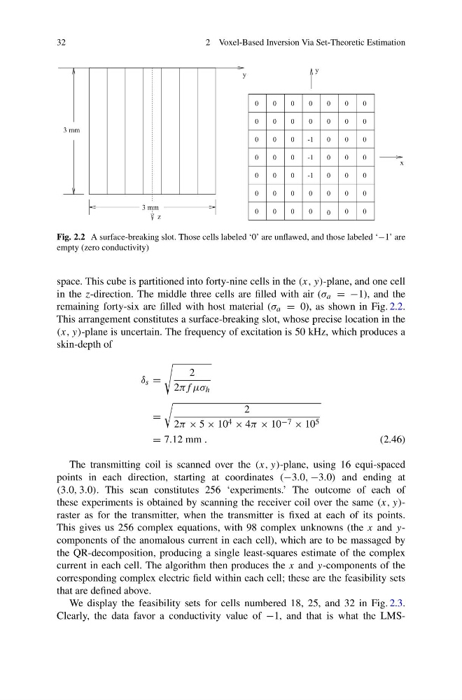
Fig. 2.2 A surface-breaking slot. Those cells labeled ‘0’ are unflawed, and those labeled ‘−1’ are
empty (zero conductivity)
space. This cube is partitioned into forty-nine cells in the (x, y)-plane, and one cell
in the z-direction. The middle three cells are filled with air (σ a = −1), and the
remaining forty-six are filled with host material (σ a = 0), as shown in Fig. 2.2.
This arrangement constitutes a surface-breaking slot, whose precise location in the
(x, y)-plane is uncertain. The frequency of excitation is 50 kHz, which produces a
skin-depth of
δ s =
2
2πf μσ h
=
2
2π × 5 × 10 4 × 4π × 10 −7 × 10 5
= 7.12 mm .
(2.46)
The transmitting coil is scanned over the (x, y)-plane, using 16 equi-spaced
points in each direction, starting at coordinates (−3.0, −3.0) and ending at
(3.0, 3.0). This scan constitutes 256 ‘experiments.’ The outcome of each of
these experiments is obtained by scanning the receiver coil over the same (x, y)raster as for the transmitter, when the transmitter is fixed at each of its points.
This gives us 256 complex equations, with 98 complex unknowns (the x and ycomponents of the anomalous current in each cell), which are to be massaged by
the QR-decomposition, producing a single least-squares estimate of the complex
current in each cell. The algorithm then produces the x and y-components of the
corresponding complex electric field within each cell; these are the feasibility sets
that are defined above.
We display the feasibility sets for cells numbered 18, 25, and 32 in Fig. 2.3.
Clearly, the data favor a conductivity value of −1, and that is what the LMS-
2 Voxel-Based Inversion Via Set-Theoretic Estimation
3 mm
3 mm
z
y
0
0
0
0
0
0
0
0
0
0
0
0
0
0
0
0
0
0
0
0
0
0
0
0
0
0
0
0
0
0
0
0
0
0
0
0
0
0
0
0
0
0
0
0
0
0
-1
-1
-1
y
x
Fig. 2.2 A surface-breaking slot. Those cells labeled ‘0’ are unflawed, and those labeled ‘−1’ are
empty (zero conductivity)
space. This cube is partitioned into forty-nine cells in the (x, y)-plane, and one cell
in the z-direction. The middle three cells are filled with air (σ a = −1), and the
remaining forty-six are filled with host material (σ a = 0), as shown in Fig. 2.2.
This arrangement constitutes a surface-breaking slot, whose precise location in the
(x, y)-plane is uncertain. The frequency of excitation is 50 kHz, which produces a
skin-depth of
δ s =
2
2πf μσ h
=
2
2π × 5 × 10 4 × 4π × 10 −7 × 10 5
= 7.12 mm .
(2.46)
The transmitting coil is scanned over the (x, y)-plane, using 16 equi-spaced
points in each direction, starting at coordinates (−3.0, −3.0) and ending at
(3.0, 3.0). This scan constitutes 256 ‘experiments.’ The outcome of each of
these experiments is obtained by scanning the receiver coil over the same (x, y)raster as for the transmitter, when the transmitter is fixed at each of its points.
This gives us 256 complex equations, with 98 complex unknowns (the x and ycomponents of the anomalous current in each cell), which are to be massaged by
the QR-decomposition, producing a single least-squares estimate of the complex
current in each cell. The algorithm then produces the x and y-components of the
corresponding complex electric field within each cell; these are the feasibility sets
that are defined above.
We display the feasibility sets for cells numbered 18, 25, and 32 in Fig. 2.3.
Clearly, the data favor a conductivity value of −1, and that is what the LMS-