

2.5 Some Examples of the Inversion Algorithm
37
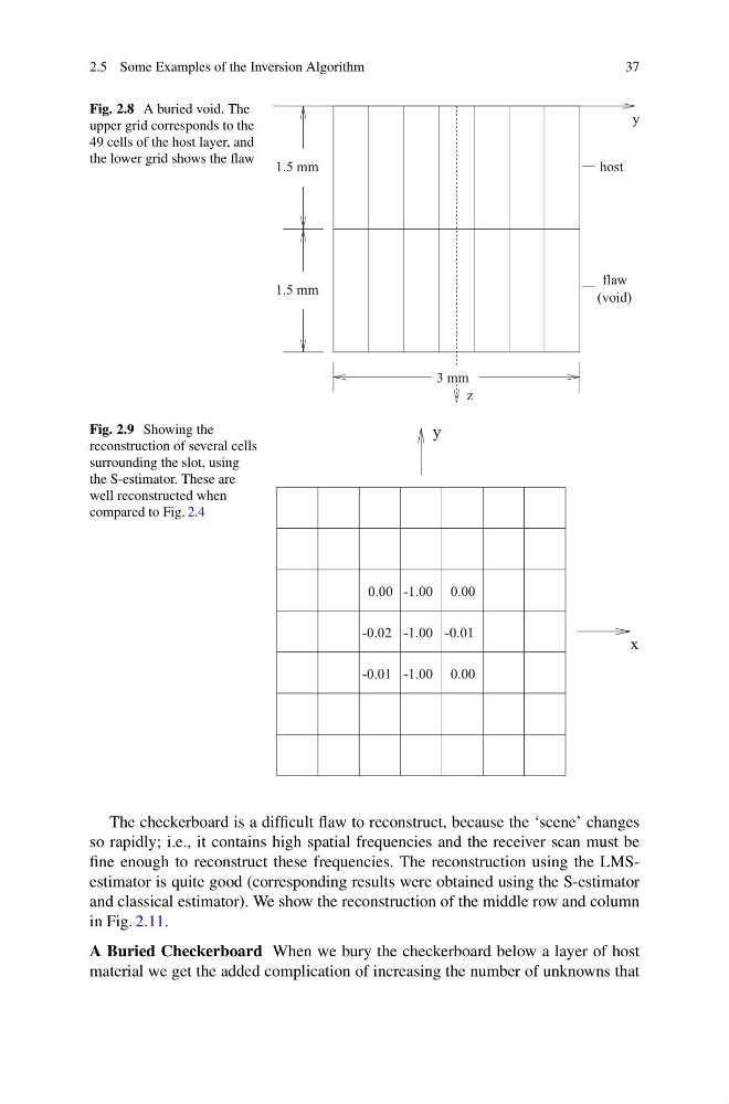
Fig. 2.8 A buried void. The
upper grid corresponds to the
49 cells of the host layer, and
the lower grid shows the flaw
3 mm
z
y
1.5 mm
1.5 mm
host
flaw
(void)
Fig. 2.9 Showing the
reconstruction of several cells
surrounding the slot, using
the S-estimator. These are
well reconstructed when
compared to Fig. 2.4
-0.02
-0.01
-0.01
0.00
0.00
0.00
-1.00
-1.00
-1.00
y
x
The checkerboard is a difficult flaw to reconstruct, because the ‘scene’ changes
so rapidly; i.e., it contains high spatial frequencies and the receiver scan must be
fine enough to reconstruct these frequencies. The reconstruction using the LMSestimator is quite good (corresponding results were obtained using the S-estimator
and classical estimator). We show the reconstruction of the middle row and column
in Fig. 2.11.
A Buried Checkerboard When we bury the checkerboard below a layer of host
material we get the added complication of increasing the number of unknowns that
37
Fig. 2.8 A buried void. The
upper grid corresponds to the
49 cells of the host layer, and
the lower grid shows the flaw
3 mm
z
y
1.5 mm
1.5 mm
host
flaw
(void)
Fig. 2.9 Showing the
reconstruction of several cells
surrounding the slot, using
the S-estimator. These are
well reconstructed when
compared to Fig. 2.4
-0.02
-0.01
-0.01
0.00
0.00
0.00
-1.00
-1.00
-1.00
y
x
The checkerboard is a difficult flaw to reconstruct, because the ‘scene’ changes
so rapidly; i.e., it contains high spatial frequencies and the receiver scan must be
fine enough to reconstruct these frequencies. The reconstruction using the LMSestimator is quite good (corresponding results were obtained using the S-estimator
and classical estimator). We show the reconstruction of the middle row and column
in Fig. 2.11.
A Buried Checkerboard When we bury the checkerboard below a layer of host
material we get the added complication of increasing the number of unknowns that