

12.8 Inverse Problems
333
where a is the length of the graphene lattice unit vector, d is the diameter of the
CNT, and b is the change in the transfer integral with change in bond length.
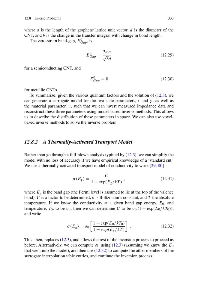
The zero-strain band-gap, E 0
Gap , is
E
0
Gap =
2t 0 a
√
3d
(12.29)
for a semiconducting CNT, and
E
0
Gap = 0
(12.30)
for metallic CNTs.
To summarize: given the various quantum factors and the solution of (12.3), we
can generate a surrogate model for the two state parameters, and γ , as well as
the material parameter, ν, such that we can invert measured impedance data and
reconstruct these three parameters using model-based inverse methods. This allows
us to describe the distribution of these parameters in space. We can also use voxelbased inverse methods to solve the inverse problem.
12.8.2 A Thermally-Activated Transport Model
Rather than go through a full-blown analysis typified by (12.3), we can simplify the
model with no loss of accuracy if we have empirical knowledge of a ‘standard cnt.’
We use a thermally activated transport model of conductivity to write [29, 80]
σ (E g ) =
C
1 + exp(E g /kT )
,
(12.31)
where E g is the band gap (the Fermi level is assumed to lie at the top of the valence
band), C is a factor to be determined, k is Boltzmann’s constant, and T the absolute
temperature. If we know the conductivity at a given band gap energy, E 0 , and
temperature, T 0 , to be σ 0 , then we can determine C to be σ 0 (1 + exp(E 0 /kT 0 )),
and write
σ (E g ) = σ 0
1 + exp(E 0 /kT 0 )
1 + exp(E g /kT )
.
(12.32)
This, then, replaces (12.3), and allows the rest of the inversion process to proceed as
before. Alternatively, we can compute σ 0 using (12.3) (assuming we know the E 0
that went into the model), and then use (12.32) to compute the other members of the
surrogate interpolation table entries, and continue the inversion process.
333
where a is the length of the graphene lattice unit vector, d is the diameter of the
CNT, and b is the change in the transfer integral with change in bond length.
The zero-strain band-gap, E 0
Gap , is
E
0
Gap =
2t 0 a
√
3d
(12.29)
for a semiconducting CNT, and
E
0
Gap = 0
(12.30)
for metallic CNTs.
To summarize: given the various quantum factors and the solution of (12.3), we
can generate a surrogate model for the two state parameters, and γ , as well as
the material parameter, ν, such that we can invert measured impedance data and
reconstruct these three parameters using model-based inverse methods. This allows
us to describe the distribution of these parameters in space. We can also use voxelbased inverse methods to solve the inverse problem.
12.8.2 A Thermally-Activated Transport Model
Rather than go through a full-blown analysis typified by (12.3), we can simplify the
model with no loss of accuracy if we have empirical knowledge of a ‘standard cnt.’
We use a thermally activated transport model of conductivity to write [29, 80]
σ (E g ) =
C
1 + exp(E g /kT )
,
(12.31)
where E g is the band gap (the Fermi level is assumed to lie at the top of the valence
band), C is a factor to be determined, k is Boltzmann’s constant, and T the absolute
temperature. If we know the conductivity at a given band gap energy, E 0 , and
temperature, T 0 , to be σ 0 , then we can determine C to be σ 0 (1 + exp(E 0 /kT 0 )),
and write
σ (E g ) = σ 0
1 + exp(E 0 /kT 0 )
1 + exp(E g /kT )
.
(12.32)
This, then, replaces (12.3), and allows the rest of the inversion process to proceed as
before. Alternatively, we can compute σ 0 using (12.3) (assuming we know the E 0
that went into the model), and then use (12.32) to compute the other members of the
surrogate interpolation table entries, and continue the inversion process.