

334
12 Carbon-Nanotube Reinforced Polymers
-550000
-500000
-450000
-400000
-350000
-300000
-250000
-200000
-150000
-100000
-50000
0
0
1
2
3
4
5
6
7
8
9
10
R
Freq(GHz)
-150000
-100000
-50000
0
50000
100000
150000
0
1
2
3
4
5
6
7
8
9
10
X
Freq(GHz)
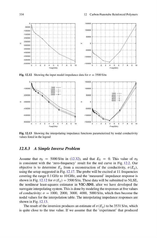
Fig. 12.12 Showing the input model impedance data for σ = 3500 S/m
-600000
-500000
-400000
-300000
-200000
-100000
0
0
1
2
3
4
5
6
7
8
9
10
R
Freq(GHz)
1000
2000
3000
4000
5000
-150000
-100000
-50000
0
50000
100000
150000
0
1
2
3
4
5
6
7
8
9
10
X
Freq(GHz)
1000
2000
3000
4000
5000
Fig. 12.13 Showing the interpolating impedance functions parameterized by nodal conductivity
values listed in the legend
12.8.3 A Simple Inverse Problem
Assume that σ 0 = 5000 S/m in (12.32), and that E 0 = 0. This value of σ 0
is consistent with the ‘zero-frequency’ result for the red curve in Fig. 12.2. Our
objective is to determine E g from a reconstruction of the conductivity, σ (E g ),
using the setup suggested in Fig. 12.17. The probe will be excited at 11 frequencies
covering the range 0.1 GHz to 10 GHz, and the ‘measured’ impedance response is
shown in Fig. 12.12 for σ (E g ) = 3500 S/m. These data will be submitted to NLSE,
the nonlinear least-squares estimator in VIC-3D®, after we have developed the
surrogate interpolating system. This is done by modeling the responses at five values
of conductivity: σ = 1000, 2000, 3000, 4000, 5000 S/m, which then become the
nodal values for the interpolation table. The interpolating impedance responses are
shown in Fig. 12.13.
The result of the inversion produces an estimate of σ (E g ) to be 3531 S/m, which
is quite close to the true value. If we assume that the ’experiment’ that produced
12 Carbon-Nanotube Reinforced Polymers
-550000
-500000
-450000
-400000
-350000
-300000
-250000
-200000
-150000
-100000
-50000
0
0
1
2
3
4
5
6
7
8
9
10
R
Freq(GHz)
-150000
-100000
-50000
0
50000
100000
150000
0
1
2
3
4
5
6
7
8
9
10
X
Freq(GHz)
Fig. 12.12 Showing the input model impedance data for σ = 3500 S/m
-600000
-500000
-400000
-300000
-200000
-100000
0
0
1
2
3
4
5
6
7
8
9
10
R
Freq(GHz)
1000
2000
3000
4000
5000
-150000
-100000
-50000
0
50000
100000
150000
0
1
2
3
4
5
6
7
8
9
10
X
Freq(GHz)
1000
2000
3000
4000
5000
Fig. 12.13 Showing the interpolating impedance functions parameterized by nodal conductivity
values listed in the legend
12.8.3 A Simple Inverse Problem
Assume that σ 0 = 5000 S/m in (12.32), and that E 0 = 0. This value of σ 0
is consistent with the ‘zero-frequency’ result for the red curve in Fig. 12.2. Our
objective is to determine E g from a reconstruction of the conductivity, σ (E g ),
using the setup suggested in Fig. 12.17. The probe will be excited at 11 frequencies
covering the range 0.1 GHz to 10 GHz, and the ‘measured’ impedance response is
shown in Fig. 12.12 for σ (E g ) = 3500 S/m. These data will be submitted to NLSE,
the nonlinear least-squares estimator in VIC-3D®, after we have developed the
surrogate interpolating system. This is done by modeling the responses at five values
of conductivity: σ = 1000, 2000, 3000, 4000, 5000 S/m, which then become the
nodal values for the interpolation table. The interpolating impedance responses are
shown in Fig. 12.13.
The result of the inversion produces an estimate of σ (E g ) to be 3531 S/m, which
is quite close to the true value. If we assume that the ’experiment’ that produced