

12.4 Quantum-Mechanical Model for Conductivity
317
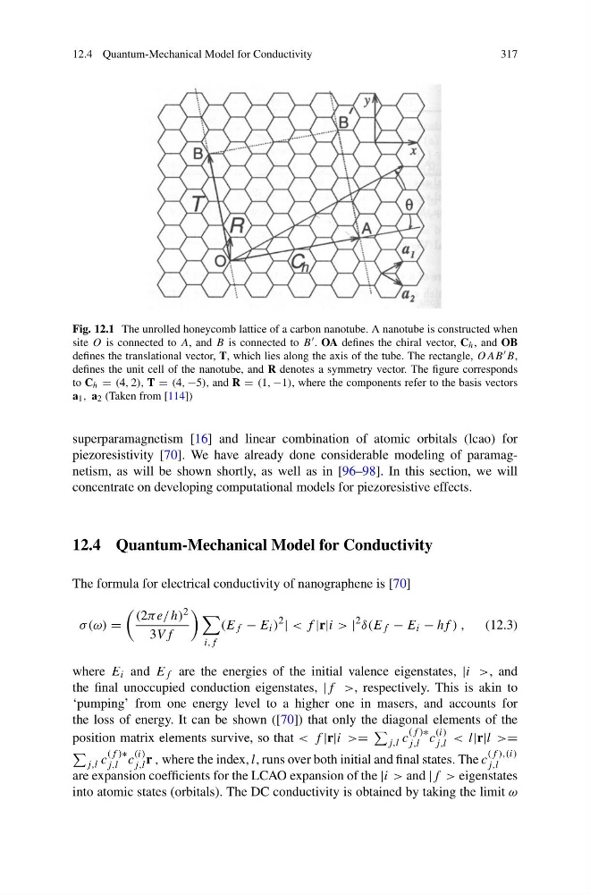
Fig. 12.1 The unrolled honeycomb lattice of a carbon nanotube. A nanotube is constructed when
site O is connected to A, and B is connected to B . OA defines the chiral vector, C h , and OB
defines the translational vector, T, which lies along the axis of the tube. The rectangle, OAB B,
defines the unit cell of the nanotube, and R denotes a symmetry vector. The figure corresponds
to C h = (4, 2), T = (4, −5), and R = (1, −1), where the components refer to the basis vectors
a 1 , a 2 (Taken from [114])
superparamagnetism [16] and linear combination of atomic orbitals (lcao) for
piezoresistivity [70]. We have already done considerable modeling of paramagnetism, as will be shown shortly, as well as in [96–98]. In this section, we will
concentrate on developing computational models for piezoresistive effects.
12.4 Quantum-Mechanical Model for Conductivity
The formula for electrical conductivity of nanographene is [70]
σ (ω) =
(2πe/h) 2
3Vf
i,f
(E f − E i )
2
| < f |r|i > |
2 δ(E f − E i − hf ) ,
(12.3)
where E i and E f are the energies of the initial valence eigenstates, |i >, and
the final unoccupied conduction eigenstates, |f >, respectively. This is akin to
‘pumping’ from one energy level to a higher one in masers, and accounts for
the loss of energy. It can be shown ([70]) that only the diagonal elements of the
position matrix elements survive, so that < f |r|i >=
j,l c
(f )∗
j,l c
(i)
j,l < l|r|l >=
j,l c
(f )∗
j,l c
(i)
j,l r , where the index, l, runs over both initial and final states. The c
(f ),(i)
j,l
are expansion coefficients for the LCAO expansion of the |i > and |f > eigenstates
into atomic states (orbitals). The DC conductivity is obtained by taking the limit ω
317
Fig. 12.1 The unrolled honeycomb lattice of a carbon nanotube. A nanotube is constructed when
site O is connected to A, and B is connected to B . OA defines the chiral vector, C h , and OB
defines the translational vector, T, which lies along the axis of the tube. The rectangle, OAB B,
defines the unit cell of the nanotube, and R denotes a symmetry vector. The figure corresponds
to C h = (4, 2), T = (4, −5), and R = (1, −1), where the components refer to the basis vectors
a 1 , a 2 (Taken from [114])
superparamagnetism [16] and linear combination of atomic orbitals (lcao) for
piezoresistivity [70]. We have already done considerable modeling of paramagnetism, as will be shown shortly, as well as in [96–98]. In this section, we will
concentrate on developing computational models for piezoresistive effects.
12.4 Quantum-Mechanical Model for Conductivity
The formula for electrical conductivity of nanographene is [70]
σ (ω) =
(2πe/h) 2
3Vf
i,f
(E f − E i )
2
| < f |r|i > |
2 δ(E f − E i − hf ) ,
(12.3)
where E i and E f are the energies of the initial valence eigenstates, |i >, and
the final unoccupied conduction eigenstates, |f >, respectively. This is akin to
‘pumping’ from one energy level to a higher one in masers, and accounts for
the loss of energy. It can be shown ([70]) that only the diagonal elements of the
position matrix elements survive, so that < f |r|i >=
j,l c
(f )∗
j,l c
(i)
j,l < l|r|l >=
j,l c
(f )∗
j,l c
(i)
j,l r , where the index, l, runs over both initial and final states. The c
(f ),(i)
j,l
are expansion coefficients for the LCAO expansion of the |i > and |f > eigenstates
into atomic states (orbitals). The DC conductivity is obtained by taking the limit ω