

11.5 Crystalline Anisotropy and TiO 2
309
17200
17250
17300
17350
17400
17450
17500
0
2
4
6
8
10
Frequency (GHz)
H (kgauss)
Spectrum for Exchange Interaction
1
2
3
4
5
6
7
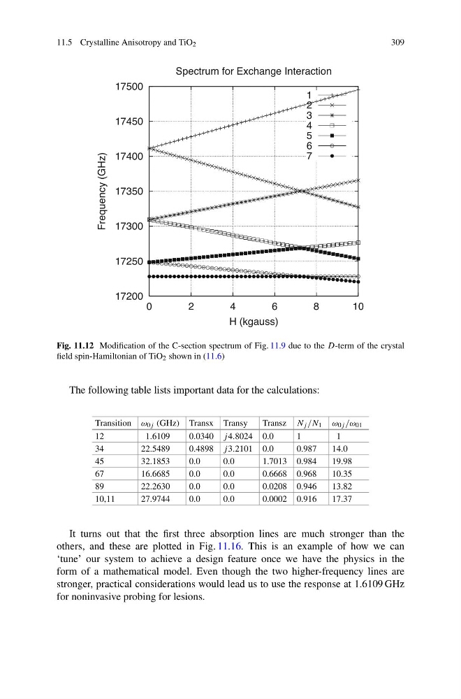
Fig. 11.12 Modification of the C-section spectrum of Fig. 11.9 due to the D-term of the crystal
field spin-Hamiltonian of TiO 2 shown in (11.6)
The following table lists important data for the calculations:
Transition ω 0j (GHz) Transx Transy
Transz N j /N 1 ω 0j /ω 01
12
1.6109
0.0340 j 4.8024 0.0
1
1
34
22.5489
0.4898 j 3.2101 0.0
0.987
14.0
45
32.1853
0.0
0.0
1.7013 0.984
19.98
67
16.6685
0.0
0.0
0.6668 0.968
10.35
89
22.2630
0.0
0.0
0.0208 0.946
13.82
10,11
27.9744
0.0
0.0
0.0002 0.916
17.37
It turns out that the first three absorption lines are much stronger than the
others, and these are plotted in Fig. 11.16. This is an example of how we can
‘tune’ our system to achieve a design feature once we have the physics in the
form of a mathematical model. Even though the two higher-frequency lines are
stronger, practical considerations would lead us to use the response at 1.6109 GHz
for noninvasive probing for lesions.
309
17200
17250
17300
17350
17400
17450
17500
0
2
4
6
8
10
Frequency (GHz)
H (kgauss)
Spectrum for Exchange Interaction
1
2
3
4
5
6
7
Fig. 11.12 Modification of the C-section spectrum of Fig. 11.9 due to the D-term of the crystal
field spin-Hamiltonian of TiO 2 shown in (11.6)
The following table lists important data for the calculations:
Transition ω 0j (GHz) Transx Transy
Transz N j /N 1 ω 0j /ω 01
12
1.6109
0.0340 j 4.8024 0.0
1
1
34
22.5489
0.4898 j 3.2101 0.0
0.987
14.0
45
32.1853
0.0
0.0
1.7013 0.984
19.98
67
16.6685
0.0
0.0
0.6668 0.968
10.35
89
22.2630
0.0
0.0
0.0208 0.946
13.82
10,11
27.9744
0.0
0.0
0.0002 0.916
17.37
It turns out that the first three absorption lines are much stronger than the
others, and these are plotted in Fig. 11.16. This is an example of how we can
‘tune’ our system to achieve a design feature once we have the physics in the
form of a mathematical model. Even though the two higher-frequency lines are
stronger, practical considerations would lead us to use the response at 1.6109 GHz
for noninvasive probing for lesions.