

11.3 Superparamagnetic Iron Oxide
297
(3/2) (1/2) (1/2) (1/2) (−1/2) (−1/2) (−1/2) (−3/2)
⎡
⎢
⎢
⎢
⎢
⎢
⎢
⎢
⎢
⎢
⎢
⎢
⎣
1.0
0.0
0.0
0.0
0.0
0.0
0.0
0.0
⎤
⎥
⎥
⎥
⎥
⎥
⎥
⎥
⎥
⎥
⎥
⎥
⎦
⎡
⎢
⎢
⎢
⎢
⎢
⎢
⎢
⎢
⎢
⎢
⎢
⎣
0.0
1.0
0.0
0.0
0.0
0.0
0.0
0.0
⎤
⎥
⎥
⎥
⎥
⎥
⎥
⎥
⎥
⎥
⎥
⎥
⎦
⎡
⎢
⎢
⎢
⎢
⎢
⎢
⎢
⎢
⎢
⎢
⎢
⎣
0.0
0.0
1.0
0.0
0.0
0.0
0.0
0.0
⎤
⎥
⎥
⎥
⎥
⎥
⎥
⎥
⎥
⎥
⎥
⎥
⎦
⎡
⎢
⎢
⎢
⎢
⎢
⎢
⎢
⎢
⎢
⎢
⎢
⎣
0.0
0.0
0.0
0.0
1.0
0.0
0.0
0.0
⎤
⎥
⎥
⎥
⎥
⎥
⎥
⎥
⎥
⎥
⎥
⎥
⎦
⎡
⎢
⎢
⎢
⎢
⎢
⎢
⎢
⎢
⎢
⎢
⎢
⎣
0.0
0.0
0.0
1.0
0.0
0.0
0.0
0.0
⎤
⎥
⎥
⎥
⎥
⎥
⎥
⎥
⎥
⎥
⎥
⎥
⎦
⎡
⎢
⎢
⎢
⎢
⎢
⎢
⎢
⎢
⎢
⎢
⎢
⎣
0.0
0.0
0.0
0.0
0.0
1.0
0.0
0.0
⎤
⎥
⎥
⎥
⎥
⎥
⎥
⎥
⎥
⎥
⎥
⎥
⎦
⎡
⎢
⎢
⎢
⎢
⎢
⎢
⎢
⎢
⎢
⎢
⎢
⎣
0.0
0.0
0.0
0.0
0.0
0.0
1.0
0.0
⎤
⎥
⎥
⎥
⎥
⎥
⎥
⎥
⎥
⎥
⎥
⎥
⎦
⎡
⎢
⎢
⎢
⎢
⎢
⎢
⎢
⎢
⎢
⎢
⎢
⎣
0.0
0.0
0.0
0.0
0.0
0.0
0.0
1.0
⎤
⎥
⎥
⎥
⎥
⎥
⎥
⎥
⎥
⎥
⎥
⎥
⎦
(• • •) (• • ◦) (• ◦ •) (◦ • •) (• ◦ ◦) (◦ • ◦) (◦ ◦ •) (◦ ◦ ◦)
,
(11.28)
where • denotes a spin-up state (parallel to the magnetic field), and ◦ denotes a
spin-down state.
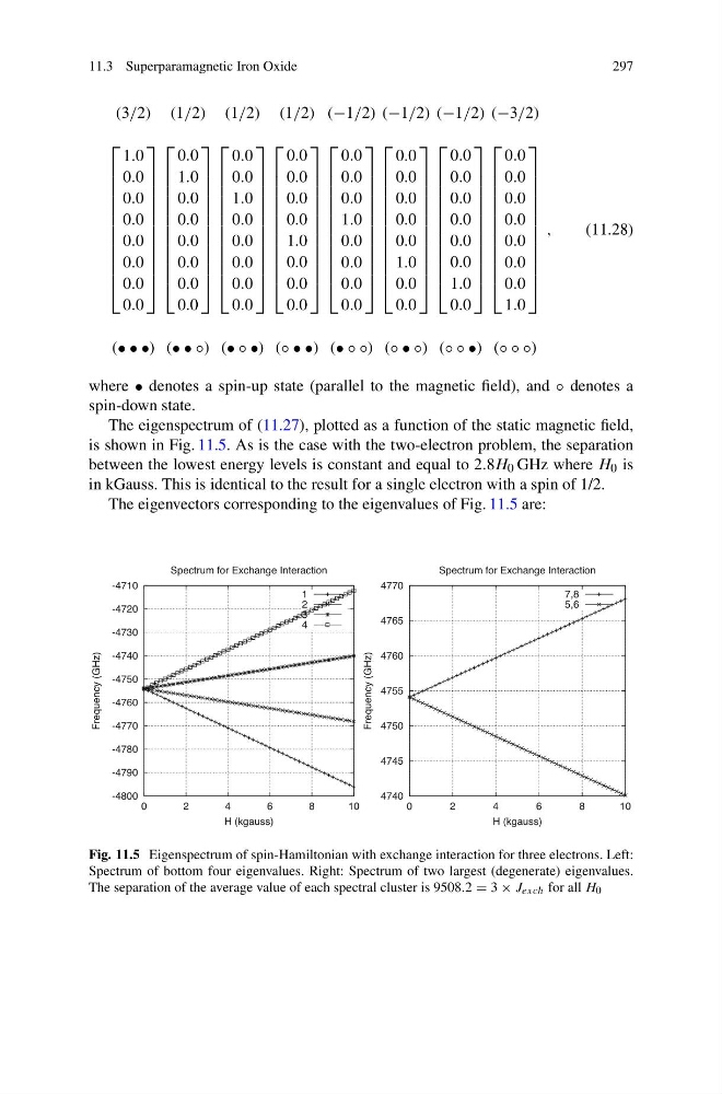
The eigenspectrum of (11.27), plotted as a function of the static magnetic field,
is shown in Fig. 11.5. As is the case with the two-electron problem, the separation
between the lowest energy levels is constant and equal to 2.8H 0 GHz where H 0 is
in kGauss. This is identical to the result for a single electron with a spin of 1/2.
The eigenvectors corresponding to the eigenvalues of Fig. 11.5 are:
-4800
-4790
-4780
-4770
-4760
-4750
-4740
-4730
-4720
-4710
0
2
4
6
8
10
Frequency (GHz)
H (kgauss)
Spectrum for Exchange Interaction
1
2
3
4
4740
4745
4750
4755
4760
4765
4770
0
2
4
6
8
10
Frequency (GHz)
H (kgauss)
Spectrum for Exchange Interaction
7,8
5,6
Fig. 11.5 Eigenspectrum of spin-Hamiltonian with exchange interaction for three electrons. Left:
Spectrum of bottom four eigenvalues. Right: Spectrum of two largest (degenerate) eigenvalues.
The separation of the average value of each spectral cluster is 9508.2 = 3 × J exch for all H 0
297
(3/2) (1/2) (1/2) (1/2) (−1/2) (−1/2) (−1/2) (−3/2)
⎡
⎢
⎢
⎢
⎢
⎢
⎢
⎢
⎢
⎢
⎢
⎢
⎣
1.0
0.0
0.0
0.0
0.0
0.0
0.0
0.0
⎤
⎥
⎥
⎥
⎥
⎥
⎥
⎥
⎥
⎥
⎥
⎥
⎦
⎡
⎢
⎢
⎢
⎢
⎢
⎢
⎢
⎢
⎢
⎢
⎢
⎣
0.0
1.0
0.0
0.0
0.0
0.0
0.0
0.0
⎤
⎥
⎥
⎥
⎥
⎥
⎥
⎥
⎥
⎥
⎥
⎥
⎦
⎡
⎢
⎢
⎢
⎢
⎢
⎢
⎢
⎢
⎢
⎢
⎢
⎣
0.0
0.0
1.0
0.0
0.0
0.0
0.0
0.0
⎤
⎥
⎥
⎥
⎥
⎥
⎥
⎥
⎥
⎥
⎥
⎥
⎦
⎡
⎢
⎢
⎢
⎢
⎢
⎢
⎢
⎢
⎢
⎢
⎢
⎣
0.0
0.0
0.0
0.0
1.0
0.0
0.0
0.0
⎤
⎥
⎥
⎥
⎥
⎥
⎥
⎥
⎥
⎥
⎥
⎥
⎦
⎡
⎢
⎢
⎢
⎢
⎢
⎢
⎢
⎢
⎢
⎢
⎢
⎣
0.0
0.0
0.0
1.0
0.0
0.0
0.0
0.0
⎤
⎥
⎥
⎥
⎥
⎥
⎥
⎥
⎥
⎥
⎥
⎥
⎦
⎡
⎢
⎢
⎢
⎢
⎢
⎢
⎢
⎢
⎢
⎢
⎢
⎣
0.0
0.0
0.0
0.0
0.0
1.0
0.0
0.0
⎤
⎥
⎥
⎥
⎥
⎥
⎥
⎥
⎥
⎥
⎥
⎥
⎦
⎡
⎢
⎢
⎢
⎢
⎢
⎢
⎢
⎢
⎢
⎢
⎢
⎣
0.0
0.0
0.0
0.0
0.0
0.0
1.0
0.0
⎤
⎥
⎥
⎥
⎥
⎥
⎥
⎥
⎥
⎥
⎥
⎥
⎦
⎡
⎢
⎢
⎢
⎢
⎢
⎢
⎢
⎢
⎢
⎢
⎢
⎣
0.0
0.0
0.0
0.0
0.0
0.0
0.0
1.0
⎤
⎥
⎥
⎥
⎥
⎥
⎥
⎥
⎥
⎥
⎥
⎥
⎦
(• • •) (• • ◦) (• ◦ •) (◦ • •) (• ◦ ◦) (◦ • ◦) (◦ ◦ •) (◦ ◦ ◦)
,
(11.28)
where • denotes a spin-up state (parallel to the magnetic field), and ◦ denotes a
spin-down state.
The eigenspectrum of (11.27), plotted as a function of the static magnetic field,
is shown in Fig. 11.5. As is the case with the two-electron problem, the separation
between the lowest energy levels is constant and equal to 2.8H 0 GHz where H 0 is
in kGauss. This is identical to the result for a single electron with a spin of 1/2.
The eigenvectors corresponding to the eigenvalues of Fig. 11.5 are:
-4800
-4790
-4780
-4770
-4760
-4750
-4740
-4730
-4720
-4710
0
2
4
6
8
10
Frequency (GHz)
H (kgauss)
Spectrum for Exchange Interaction
1
2
3
4
4740
4745
4750
4755
4760
4765
4770
0
2
4
6
8
10
Frequency (GHz)
H (kgauss)
Spectrum for Exchange Interaction
7,8
5,6
Fig. 11.5 Eigenspectrum of spin-Hamiltonian with exchange interaction for three electrons. Left:
Spectrum of bottom four eigenvalues. Right: Spectrum of two largest (degenerate) eigenvalues.
The separation of the average value of each spectral cluster is 9508.2 = 3 × J exch for all H 0