

1.4 Example: Raster Scan at Three Frequencies
17
Table 1.1 Coil parameters
for Example 1
Parameter
Transmit Receive
Inner radius (mm) 15.0
0.25
Outer radius (mm) 25.0
0.50
Height (mm)
3.0
1.0
Turns
100
100
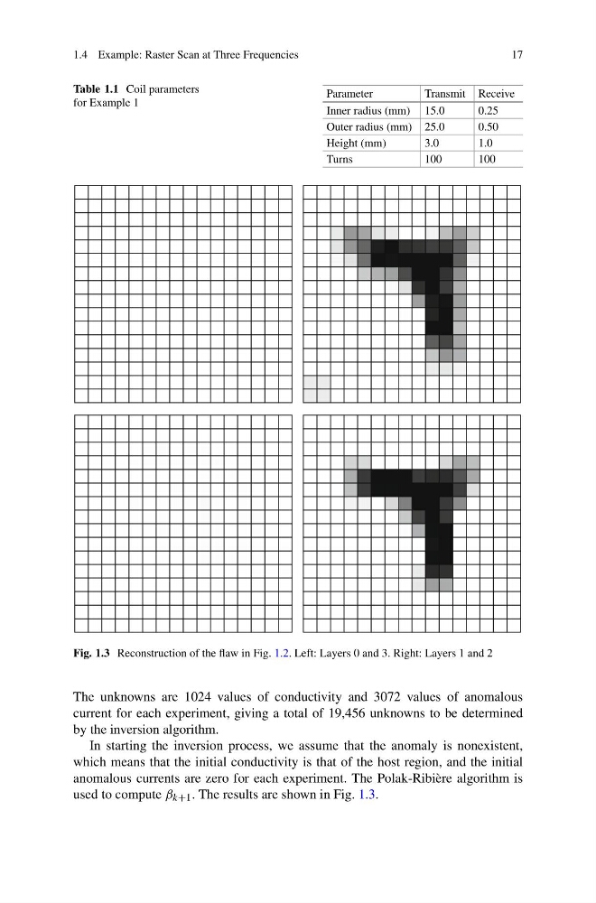
Fig. 1.3 Reconstruction of the flaw in Fig. 1.2. Left: Layers 0 and 3. Right: Layers 1 and 2
The unknowns are 1024 values of conductivity and 3072 values of anomalous
current for each experiment, giving a total of 19,456 unknowns to be determined
by the inversion algorithm.
In starting the inversion process, we assume that the anomaly is nonexistent,
which means that the initial conductivity is that of the host region, and the initial
anomalous currents are zero for each experiment. The Polak-Ribière algorithm is
used to compute β k+1 . The results are shown in Fig. 1.3.
17
Table 1.1 Coil parameters
for Example 1
Parameter
Transmit Receive
Inner radius (mm) 15.0
0.25
Outer radius (mm) 25.0
0.50
Height (mm)
3.0
1.0
Turns
100
100
Fig. 1.3 Reconstruction of the flaw in Fig. 1.2. Left: Layers 0 and 3. Right: Layers 1 and 2
The unknowns are 1024 values of conductivity and 3072 values of anomalous
current for each experiment, giving a total of 19,456 unknowns to be determined
by the inversion algorithm.
In starting the inversion process, we assume that the anomaly is nonexistent,
which means that the initial conductivity is that of the host region, and the initial
anomalous currents are zero for each experiment. The Polak-Ribière algorithm is
used to compute β k+1 . The results are shown in Fig. 1.3.