

18
1 A Bilinear Conjugate-Gradient Inversion Algorithm
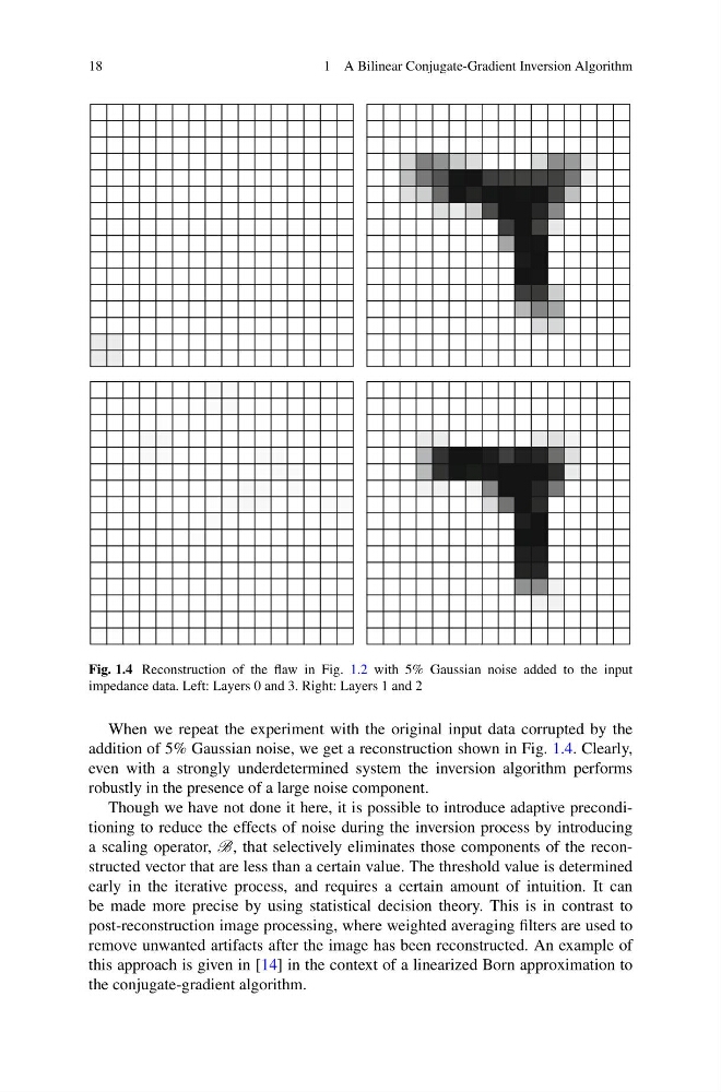
Fig. 1.4 Reconstruction of the flaw in Fig. 1.2 with 5% Gaussian noise added to the input
impedance data. Left: Layers 0 and 3. Right: Layers 1 and 2
When we repeat the experiment with the original input data corrupted by the
addition of 5% Gaussian noise, we get a reconstruction shown in Fig. 1.4. Clearly,
even with a strongly underdetermined system the inversion algorithm performs
robustly in the presence of a large noise component.
Though we have not done it here, it is possible to introduce adaptive preconditioning to reduce the effects of noise during the inversion process by introducing
a scaling operator, B, that selectively eliminates those components of the reconstructed vector that are less than a certain value. The threshold value is determined
early in the iterative process, and requires a certain amount of intuition. It can
be made more precise by using statistical decision theory. This is in contrast to
post-reconstruction image processing, where weighted averaging filters are used to
remove unwanted artifacts after the image has been reconstructed. An example of
this approach is given in [14] in the context of a linearized Born approximation to
the conjugate-gradient algorithm.
1 A Bilinear Conjugate-Gradient Inversion Algorithm
Fig. 1.4 Reconstruction of the flaw in Fig. 1.2 with 5% Gaussian noise added to the input
impedance data. Left: Layers 0 and 3. Right: Layers 1 and 2
When we repeat the experiment with the original input data corrupted by the
addition of 5% Gaussian noise, we get a reconstruction shown in Fig. 1.4. Clearly,
even with a strongly underdetermined system the inversion algorithm performs
robustly in the presence of a large noise component.
Though we have not done it here, it is possible to introduce adaptive preconditioning to reduce the effects of noise during the inversion process by introducing
a scaling operator, B, that selectively eliminates those components of the reconstructed vector that are less than a certain value. The threshold value is determined
early in the iterative process, and requires a certain amount of intuition. It can
be made more precise by using statistical decision theory. This is in contrast to
post-reconstruction image processing, where weighted averaging filters are used to
remove unwanted artifacts after the image has been reconstructed. An example of
this approach is given in [14] in the context of a linearized Born approximation to
the conjugate-gradient algorithm.