

16
1 A Bilinear Conjugate-Gradient Inversion Algorithm
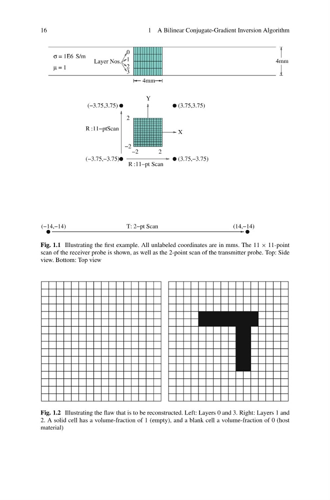
Fig. 1.1 Illustrating the first example. All unlabeled coordinates are in mms. The 11 × 11-point
scan of the receiver probe is shown, as well as the 2-point scan of the transmitter probe. Top: Side
view. Bottom: Top view
Fig. 1.2 Illustrating the flaw that is to be reconstructed. Left: Layers 0 and 3. Right: Layers 1 and
2. A solid cell has a volume-fraction of 1 (empty), and a blank cell a volume-fraction of 0 (host
material)
1 A Bilinear Conjugate-Gradient Inversion Algorithm
Fig. 1.1 Illustrating the first example. All unlabeled coordinates are in mms. The 11 × 11-point
scan of the receiver probe is shown, as well as the 2-point scan of the transmitter probe. Top: Side
view. Bottom: Top view
Fig. 1.2 Illustrating the flaw that is to be reconstructed. Left: Layers 0 and 3. Right: Layers 1 and
2. A solid cell has a volume-fraction of 1 (empty), and a blank cell a volume-fraction of 0 (host
material)