

268
10 Characterization of Atherosclerotic Lesions by Inversion of Eddy-. . .
in
Z
W
z 11 − z 12
z 12
− 12
R 0
L 0
Z W
z 22 z
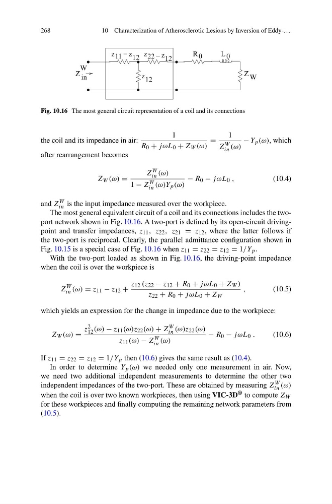
Fig. 10.16 The most general circuit representation of a coil and its connections
the coil and its impedance in air:
1
R 0 + jωL 0 + Z W (ω)
=
1
Z W
in (ω)
− Y p (ω), which
after rearrangement becomes
Z W (ω) =
Z W
in (ω)
1 − Z W
in (ω)Y p (ω)
− R 0 − jωL 0 ,
(10.4)
and Z W
in is the input impedance measured over the workpiece.
The most general equivalent circuit of a coil and its connections includes the twoport network shown in Fig. 10.16. A two-port is defined by its open-circuit drivingpoint and transfer impedances, z 11 , z 22 , z 21 = z 12 , where the latter follows if
the two-port is reciprocal. Clearly, the parallel admittance configuration shown in
Fig. 10.15 is a special case of Fig. 10.16 when z 11 = z 22 = z 12 = 1/Y p .
With the two-port loaded as shown in Fig. 10.16, the driving-point impedance
when the coil is over the workpiece is
Z
W
in (ω) = z 11 − z 12 +
z 12 (z 22 − z 12 + R 0 + jωL 0 + Z W )
z 22 + R 0 + jωL 0 + Z W
,
(10.5)
which yields an expression for the change in impedance due to the workpiece:
Z W (ω) =
z 2
12 (ω) − z 11 (ω)z 22 (ω) + Z W
in (ω)z 22 (ω)
z 11 (ω) − Z W
in (ω)
− R 0 − jωL 0 .
(10.6)
If z 11 = z 22 = z 12 = 1/Y p then (10.6) gives the same result as (10.4).
In order to determine Y p (ω) we needed only one measurement in air. Now,
we need two additional independent measurements to determine the other two
independent impedances of the two-port. These are obtained by measuring Z W
in (ω)
when the coil is over two known workpieces, then using VIC-3D ® to compute Z W
for these workpieces and finally computing the remaining network parameters from
(10.5).
10 Characterization of Atherosclerotic Lesions by Inversion of Eddy-. . .
in
Z
W
z 11 − z 12
z 12
− 12
R 0
L 0
Z W
z 22 z
Fig. 10.16 The most general circuit representation of a coil and its connections
the coil and its impedance in air:
1
R 0 + jωL 0 + Z W (ω)
=
1
Z W
in (ω)
− Y p (ω), which
after rearrangement becomes
Z W (ω) =
Z W
in (ω)
1 − Z W
in (ω)Y p (ω)
− R 0 − jωL 0 ,
(10.4)
and Z W
in is the input impedance measured over the workpiece.
The most general equivalent circuit of a coil and its connections includes the twoport network shown in Fig. 10.16. A two-port is defined by its open-circuit drivingpoint and transfer impedances, z 11 , z 22 , z 21 = z 12 , where the latter follows if
the two-port is reciprocal. Clearly, the parallel admittance configuration shown in
Fig. 10.15 is a special case of Fig. 10.16 when z 11 = z 22 = z 12 = 1/Y p .
With the two-port loaded as shown in Fig. 10.16, the driving-point impedance
when the coil is over the workpiece is
Z
W
in (ω) = z 11 − z 12 +
z 12 (z 22 − z 12 + R 0 + jωL 0 + Z W )
z 22 + R 0 + jωL 0 + Z W
,
(10.5)
which yields an expression for the change in impedance due to the workpiece:
Z W (ω) =
z 2
12 (ω) − z 11 (ω)z 22 (ω) + Z W
in (ω)z 22 (ω)
z 11 (ω) − Z W
in (ω)
− R 0 − jωL 0 .
(10.6)
If z 11 = z 22 = z 12 = 1/Y p then (10.6) gives the same result as (10.4).
In order to determine Y p (ω) we needed only one measurement in air. Now,
we need two additional independent measurements to determine the other two
independent impedances of the two-port. These are obtained by measuring Z W
in (ω)
when the coil is over two known workpieces, then using VIC-3D ® to compute Z W
for these workpieces and finally computing the remaining network parameters from
(10.5).