

10.7 Determining Coil Parameters
267
3.31e-07
3.32e-07
3.33e-07
3.34e-07
3.35e-07
3.36e-07
3.37e-07
3.38e-07
3.39e-07
8.8
9
9.2
9.4
9.6
9.8
10
Resistance (Ohms)
Frequency (E9)
Frequency Response of Probe in Freespace at 10GHz
10
10.2
10.4
10.6
10.8
11
11.2
11.4
8.8
9
9.2
9.4
9.6
9.8
10
Reactance (Ohms)
Frequency (E9)
Frequency Response of Probe in Freespace at 10GHz
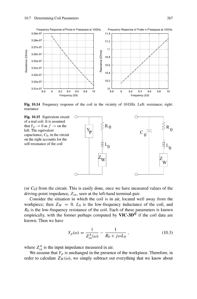
Fig. 10.14 Frequency response of the coil in the vicinity of 10 GHz. Left: resistance; right:
reactance
Fig. 10.15 Equivalent circuit
of a real coil. It is assumed
that Y p → 0 as f → on the
left. The equivalent
capacitance, C 0 , in the circuit
on the right accounts for the
self-resonance of the coil
Y
P
Z
W
W
Z
R
L
C
R
L
0
0
0
0
0
(or C 0 ) from the circuit. This is easily done, once we have measured values of the
driving-point impedance, Z in , seen at the left-hand terminal-pair.
Consider the situation in which the coil is in air, located well away from the
workpiece; then Z W = 0. L 0 is the low-frequency inductance of the coil, and
R 0 is the low-frequency resistance of the coil. Each of these parameters is known
empirically, with the former perhaps computed by VIC-3D ® if the coil data are
known. Then we have
Y p (ω) =
1
Z A
in (ω)
−
1
R 0 + jωL 0
,
(10.3)
where Z A
in is the input impedance measured in air.
We assume that Y p is unchanged in the presence of the workpiece. Therefore, in
order to calculate Z W (ω), we simply subtract out everything that we know about
267
3.31e-07
3.32e-07
3.33e-07
3.34e-07
3.35e-07
3.36e-07
3.37e-07
3.38e-07
3.39e-07
8.8
9
9.2
9.4
9.6
9.8
10
Resistance (Ohms)
Frequency (E9)
Frequency Response of Probe in Freespace at 10GHz
10
10.2
10.4
10.6
10.8
11
11.2
11.4
8.8
9
9.2
9.4
9.6
9.8
10
Reactance (Ohms)
Frequency (E9)
Frequency Response of Probe in Freespace at 10GHz
Fig. 10.14 Frequency response of the coil in the vicinity of 10 GHz. Left: resistance; right:
reactance
Fig. 10.15 Equivalent circuit
of a real coil. It is assumed
that Y p → 0 as f → on the
left. The equivalent
capacitance, C 0 , in the circuit
on the right accounts for the
self-resonance of the coil
Y
P
Z
W
W
Z
R
L
C
R
L
0
0
0
0
0
(or C 0 ) from the circuit. This is easily done, once we have measured values of the
driving-point impedance, Z in , seen at the left-hand terminal-pair.
Consider the situation in which the coil is in air, located well away from the
workpiece; then Z W = 0. L 0 is the low-frequency inductance of the coil, and
R 0 is the low-frequency resistance of the coil. Each of these parameters is known
empirically, with the former perhaps computed by VIC-3D ® if the coil data are
known. Then we have
Y p (ω) =
1
Z A
in (ω)
−
1
R 0 + jωL 0
,
(10.3)
where Z A
in is the input impedance measured in air.
We assume that Y p is unchanged in the presence of the workpiece. Therefore, in
order to calculate Z W (ω), we simply subtract out everything that we know about