

254
10 Characterization of Atherosclerotic Lesions by Inversion of Eddy-. . .
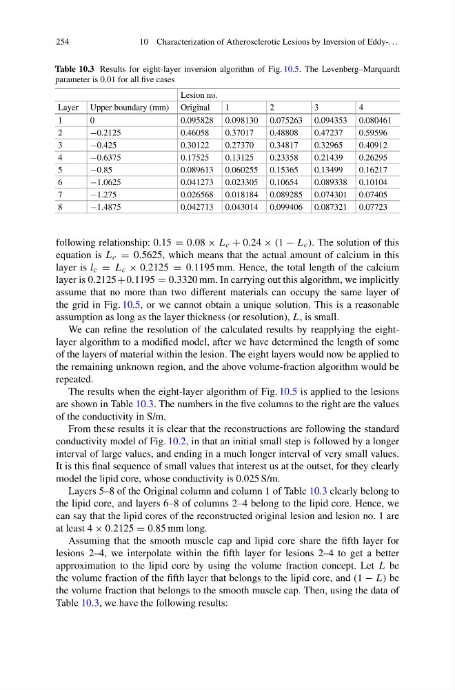
Table 10.3 Results for eight-layer inversion algorithm of Fig. 10.5. The Levenberg–Marquardt
parameter is 0.01 for all five cases
Lesion no.
Layer Upper boundary (mm) Original
1
2
3
4
1
0
0.095828 0.098130 0.075263 0.094353 0.080461
2
−0.2125
0.46058
0.37017
0.48808
0.47237
0.59596
3
−0.425
0.30122
0.27370
0.34817
0.32965
0.40912
4
−0.6375
0.17525
0.13125
0.23358
0.21439
0.26295
5
−0.85
0.089613 0.060255 0.15365
0.13499
0.16217
6
−1.0625
0.041273 0.023305 0.10654
0.089338 0.10104
7
−1.275
0.026568 0.018184 0.089285 0.074301 0.07405
8
−1.4875
0.042713 0.043014 0.099406 0.087321 0.07723
following relationship: 0.15 = 0.08 × L c + 0.24 × (1 − L c ). The solution of this
equation is L c = 0.5625, which means that the actual amount of calcium in this
layer is l c = L c × 0.2125 = 0.1195 mm. Hence, the total length of the calcium
layer is 0.2125+0.1195 = 0.3320 mm. In carrying out this algorithm, we implicitly
assume that no more than two different materials can occupy the same layer of
the grid in Fig. 10.5, or we cannot obtain a unique solution. This is a reasonable
assumption as long as the layer thickness (or resolution), L, is small.
We can refine the resolution of the calculated results by reapplying the eightlayer algorithm to a modified model, after we have determined the length of some
of the layers of material within the lesion. The eight layers would now be applied to
the remaining unknown region, and the above volume-fraction algorithm would be
repeated.
The results when the eight-layer algorithm of Fig. 10.5 is applied to the lesions
are shown in Table 10.3. The numbers in the five columns to the right are the values
of the conductivity in S/m.
From these results it is clear that the reconstructions are following the standard
conductivity model of Fig. 10.2, in that an initial small step is followed by a longer
interval of large values, and ending in a much longer interval of very small values.
It is this final sequence of small values that interest us at the outset, for they clearly
model the lipid core, whose conductivity is 0.025 S/m.
Layers 5–8 of the Original column and column 1 of Table 10.3 clearly belong to
the lipid core, and layers 6–8 of columns 2–4 belong to the lipid core. Hence, we
can say that the lipid cores of the reconstructed original lesion and lesion no. 1 are
at least 4 × 0.2125 = 0.85 mm long.
Assuming that the smooth muscle cap and lipid core share the fifth layer for
lesions 2–4, we interpolate within the fifth layer for lesions 2–4 to get a better
approximation to the lipid core by using the volume fraction concept. Let L be
the volume fraction of the fifth layer that belongs to the lipid core, and (1 − L) be
the volume fraction that belongs to the smooth muscle cap. Then, using the data of
Table 10.3, we have the following results:
10 Characterization of Atherosclerotic Lesions by Inversion of Eddy-. . .
Table 10.3 Results for eight-layer inversion algorithm of Fig. 10.5. The Levenberg–Marquardt
parameter is 0.01 for all five cases
Lesion no.
Layer Upper boundary (mm) Original
1
2
3
4
1
0
0.095828 0.098130 0.075263 0.094353 0.080461
2
−0.2125
0.46058
0.37017
0.48808
0.47237
0.59596
3
−0.425
0.30122
0.27370
0.34817
0.32965
0.40912
4
−0.6375
0.17525
0.13125
0.23358
0.21439
0.26295
5
−0.85
0.089613 0.060255 0.15365
0.13499
0.16217
6
−1.0625
0.041273 0.023305 0.10654
0.089338 0.10104
7
−1.275
0.026568 0.018184 0.089285 0.074301 0.07405
8
−1.4875
0.042713 0.043014 0.099406 0.087321 0.07723
following relationship: 0.15 = 0.08 × L c + 0.24 × (1 − L c ). The solution of this
equation is L c = 0.5625, which means that the actual amount of calcium in this
layer is l c = L c × 0.2125 = 0.1195 mm. Hence, the total length of the calcium
layer is 0.2125+0.1195 = 0.3320 mm. In carrying out this algorithm, we implicitly
assume that no more than two different materials can occupy the same layer of
the grid in Fig. 10.5, or we cannot obtain a unique solution. This is a reasonable
assumption as long as the layer thickness (or resolution), L, is small.
We can refine the resolution of the calculated results by reapplying the eightlayer algorithm to a modified model, after we have determined the length of some
of the layers of material within the lesion. The eight layers would now be applied to
the remaining unknown region, and the above volume-fraction algorithm would be
repeated.
The results when the eight-layer algorithm of Fig. 10.5 is applied to the lesions
are shown in Table 10.3. The numbers in the five columns to the right are the values
of the conductivity in S/m.
From these results it is clear that the reconstructions are following the standard
conductivity model of Fig. 10.2, in that an initial small step is followed by a longer
interval of large values, and ending in a much longer interval of very small values.
It is this final sequence of small values that interest us at the outset, for they clearly
model the lipid core, whose conductivity is 0.025 S/m.
Layers 5–8 of the Original column and column 1 of Table 10.3 clearly belong to
the lipid core, and layers 6–8 of columns 2–4 belong to the lipid core. Hence, we
can say that the lipid cores of the reconstructed original lesion and lesion no. 1 are
at least 4 × 0.2125 = 0.85 mm long.
Assuming that the smooth muscle cap and lipid core share the fifth layer for
lesions 2–4, we interpolate within the fifth layer for lesions 2–4 to get a better
approximation to the lipid core by using the volume fraction concept. Let L be
the volume fraction of the fifth layer that belongs to the lipid core, and (1 − L) be
the volume fraction that belongs to the smooth muscle cap. Then, using the data of
Table 10.3, we have the following results: