

252
10 Characterization of Atherosclerotic Lesions by Inversion of Eddy-. . .
0.002
0.004
0.006
0.008
0.01
0.012
0.014
0.016
9.5 9.55 9.6 9.65 9.7 9.75 9.8 9.85 9.9 9.95 10
Resistance (Ohms)
Frequency (E10)
Frequency Response of Lesions
original
variation 1
variation 2
variation 3
variation 4
-0.005
0
0.005
0.01
0.015
0.02
9.5 9.55 9.6 9.65 9.7 9.75 9.8 9.85 9.9 9.95 10
Reactance (Ohms)
Frequency (E10)
Frequency Response of Lesions
original
variation 1
variation 2
variation 3
variation 4
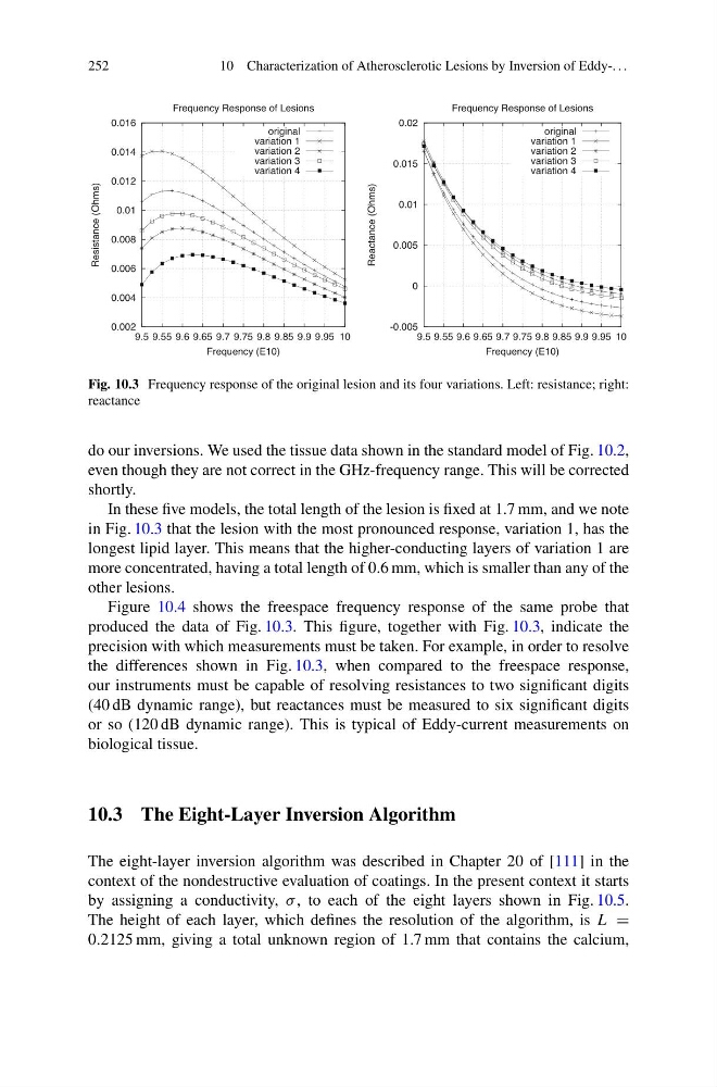
Fig. 10.3 Frequency response of the original lesion and its four variations. Left: resistance; right:
reactance
do our inversions. We used the tissue data shown in the standard model of Fig. 10.2,
even though they are not correct in the GHz-frequency range. This will be corrected
shortly.
In these five models, the total length of the lesion is fixed at 1.7 mm, and we note
in Fig. 10.3 that the lesion with the most pronounced response, variation 1, has the
longest lipid layer. This means that the higher-conducting layers of variation 1 are
more concentrated, having a total length of 0.6 mm, which is smaller than any of the
other lesions.
Figure 10.4 shows the freespace frequency response of the same probe that
produced the data of Fig. 10.3. This figure, together with Fig. 10.3, indicate the
precision with which measurements must be taken. For example, in order to resolve
the differences shown in Fig. 10.3, when compared to the freespace response,
our instruments must be capable of resolving resistances to two significant digits
(40 dB dynamic range), but reactances must be measured to six significant digits
or so (120 dB dynamic range). This is typical of Eddy-current measurements on
biological tissue.
10.3 The Eight-Layer Inversion Algorithm
The eight-layer inversion algorithm was described in Chapter 20 of [111] in the
context of the nondestructive evaluation of coatings. In the present context it starts
by assigning a conductivity, σ , to each of the eight layers shown in Fig. 10.5.
The height of each layer, which defines the resolution of the algorithm, is L =
0.2125 mm, giving a total unknown region of 1.7 mm that contains the calcium,
10 Characterization of Atherosclerotic Lesions by Inversion of Eddy-. . .
0.002
0.004
0.006
0.008
0.01
0.012
0.014
0.016
9.5 9.55 9.6 9.65 9.7 9.75 9.8 9.85 9.9 9.95 10
Resistance (Ohms)
Frequency (E10)
Frequency Response of Lesions
original
variation 1
variation 2
variation 3
variation 4
-0.005
0
0.005
0.01
0.015
0.02
9.5 9.55 9.6 9.65 9.7 9.75 9.8 9.85 9.9 9.95 10
Reactance (Ohms)
Frequency (E10)
Frequency Response of Lesions
original
variation 1
variation 2
variation 3
variation 4
Fig. 10.3 Frequency response of the original lesion and its four variations. Left: resistance; right:
reactance
do our inversions. We used the tissue data shown in the standard model of Fig. 10.2,
even though they are not correct in the GHz-frequency range. This will be corrected
shortly.
In these five models, the total length of the lesion is fixed at 1.7 mm, and we note
in Fig. 10.3 that the lesion with the most pronounced response, variation 1, has the
longest lipid layer. This means that the higher-conducting layers of variation 1 are
more concentrated, having a total length of 0.6 mm, which is smaller than any of the
other lesions.
Figure 10.4 shows the freespace frequency response of the same probe that
produced the data of Fig. 10.3. This figure, together with Fig. 10.3, indicate the
precision with which measurements must be taken. For example, in order to resolve
the differences shown in Fig. 10.3, when compared to the freespace response,
our instruments must be capable of resolving resistances to two significant digits
(40 dB dynamic range), but reactances must be measured to six significant digits
or so (120 dB dynamic range). This is typical of Eddy-current measurements on
biological tissue.
10.3 The Eight-Layer Inversion Algorithm
The eight-layer inversion algorithm was described in Chapter 20 of [111] in the
context of the nondestructive evaluation of coatings. In the present context it starts
by assigning a conductivity, σ , to each of the eight layers shown in Fig. 10.5.
The height of each layer, which defines the resolution of the algorithm, is L =
0.2125 mm, giving a total unknown region of 1.7 mm that contains the calcium,