

246
9 High-Dimension Model Representation via Sparse GridTechniques
-0.00025
-0.0002
-0.00015
-0.0001
-5e-05
0
5e-05
0.0001
0.00015
0.0002
0.00025
-100
-50
0
50
100
Resistance (Ohms)
Probe Position (mils)
-0.0008
-0.0006
-0.0004
-0.0002
0
0.0002
0.0004
0.0006
0.0008
-100
-50
0
50
100
Reactance (Ohms)
Probe Position (mils)
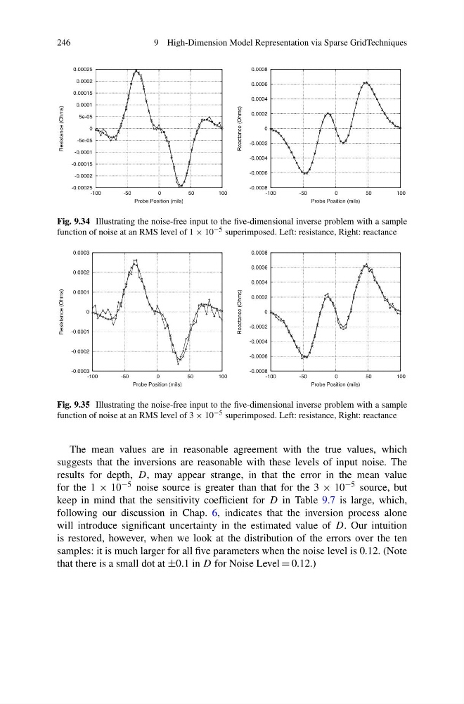
Fig. 9.34 Illustrating the noise-free input to the five-dimensional inverse problem with a sample
function of noise at an RMS level of 1 × 10 −5 superimposed. Left: resistance, Right: reactance
-0.0003
-0.0002
-0.0001
0
0.0001
0.0002
0.0003
-100
-50
0
50
100
Resistance (Ohms)
Probe Position (mils)
-0.0008
-0.0006
-0.0004
-0.0002
0
0.0002
0.0004
0.0006
0.0008
-100
-50
0
50
100
Reactance (Ohms)
Probe Position (mils)
Fig. 9.35 Illustrating the noise-free input to the five-dimensional inverse problem with a sample
function of noise at an RMS level of 3 × 10 −5 superimposed. Left: resistance, Right: reactance
The mean values are in reasonable agreement with the true values, which
suggests that the inversions are reasonable with these levels of input noise. The
results for depth, D, may appear strange, in that the error in the mean value
for the 1 × 10 −5 noise source is greater than that for the 3 × 10 −5 source, but
keep in mind that the sensitivity coefficient for D in Table 9.7 is large, which,
following our discussion in Chap. 6, indicates that the inversion process alone
will introduce significant uncertainty in the estimated value of D. Our intuition
is restored, however, when we look at the distribution of the errors over the ten
samples: it is much larger for all five parameters when the noise level is 0.12. (Note
that there is a small dot at ±0.1 in D for Noise Level = 0.12.)
9 High-Dimension Model Representation via Sparse GridTechniques
-0.00025
-0.0002
-0.00015
-0.0001
-5e-05
0
5e-05
0.0001
0.00015
0.0002
0.00025
-100
-50
0
50
100
Resistance (Ohms)
Probe Position (mils)
-0.0008
-0.0006
-0.0004
-0.0002
0
0.0002
0.0004
0.0006
0.0008
-100
-50
0
50
100
Reactance (Ohms)
Probe Position (mils)
Fig. 9.34 Illustrating the noise-free input to the five-dimensional inverse problem with a sample
function of noise at an RMS level of 1 × 10 −5 superimposed. Left: resistance, Right: reactance
-0.0003
-0.0002
-0.0001
0
0.0001
0.0002
0.0003
-100
-50
0
50
100
Resistance (Ohms)
Probe Position (mils)
-0.0008
-0.0006
-0.0004
-0.0002
0
0.0002
0.0004
0.0006
0.0008
-100
-50
0
50
100
Reactance (Ohms)
Probe Position (mils)
Fig. 9.35 Illustrating the noise-free input to the five-dimensional inverse problem with a sample
function of noise at an RMS level of 3 × 10 −5 superimposed. Left: resistance, Right: reactance
The mean values are in reasonable agreement with the true values, which
suggests that the inversions are reasonable with these levels of input noise. The
results for depth, D, may appear strange, in that the error in the mean value
for the 1 × 10 −5 noise source is greater than that for the 3 × 10 −5 source, but
keep in mind that the sensitivity coefficient for D in Table 9.7 is large, which,
following our discussion in Chap. 6, indicates that the inversion process alone
will introduce significant uncertainty in the estimated value of D. Our intuition
is restored, however, when we look at the distribution of the errors over the ten
samples: it is much larger for all five parameters when the noise level is 0.12. (Note
that there is a small dot at ±0.1 in D for Noise Level = 0.12.)