

9.10 Noisy Data and Uncertainty Propagation
245
Table 9.7 Inversion results for the five-dimensional problem at level 4 with two different
interpolation tables for NLSE
Test
Size (NLSE)
Level
No. Cal.
No. Nodes
φ
No. Pts.
1
4 × 4 × 4 × 4 × 4
4
311
1024
0.639(−5)
87
2
4 × 4 × 6 × 4 × 4
4
311
1536
0.578(−5)
78
Test
LO/Sensit
Θ/Sensit
Ψ /Sensit
L/Sensit
D/Sensit
1
3.5/2.24(−2)
5.46(−2)/4.17(−2)
20.4/0.47
1.99/4.25(−3)
2.98/0.28
2
3.5/2.02(−2)
0.11/3.71(−2)
21.51/0.36
1.99/3.83(−3)
2.99/0.25
-0.00025
-0.0002
-0.00015
-0.0001
-5e-05
0
5e-05
0.0001
0.00015
0.0002
0.00025
-100
-50
0
50
100
Resistance (Ohms)
Probe Position (mils)
-0.0008
-0.0006
-0.0004
-0.0002
0
0.0002
0.0004
0.0006
0.0008
-100
-50
0
50
100
Reactance (Ohms)
Probe Position (mils)
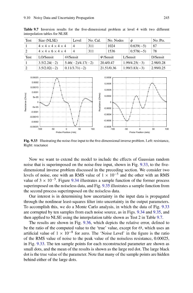
Fig. 9.33 Illustrating the noise-free input to the five-dimensional inverse problem. Left: resistance,
Right: reactance
Now we want to extend the model to include the effects of Gaussian random
noise that is superimposed on the noise-free input, shown in Fig. 9.33, to the fivedimensional inverse problem discussed in the preceding section. We consider two
levels of noise, one with an RMS value of 1 × 10 −5 and the other with an RMS
value of 3 × 10 −5 . Figure 9.34 illustrates a sample function of the former process
superimposed on the noiseless data, and Fig. 9.35 illustrates a sample function from
the second process superimposed on the noiseless data.
Our interest is in determining how uncertainty in the input data is propagated
through the nonlinear least-squares filter into uncertainty in the output parameters.
To accomplish this, we do a Monte Carlo analysis, in which the data of Fig. 9.33
are corrupted by ten samples from each noise source, as in Figs. 9.34 and 9.35, and
then applied to NLSE using the interpolation table shown as Test 2 in Table 9.7.
The results are shown in Fig. 9.36, which depicts the relative error, defined to
be the ratio of the computed value to the ‘true’ value, except for Θ, which uses an
artificial value of 1 × 10 −8 for zero. The ‘Noise Level’ in the figure is the ratio
of the RMS value of noise to the peak value of the noiseless resistance, 0.00025,
in Fig. 9.33. The ten sample points for each reconstructed parameter are shown as
small dots, and the mean of the results is shown as the large red dot. The large black
dot is the true value of the parameter. Note that many of the sample points are hidden
behind either of the large dots.
245
Table 9.7 Inversion results for the five-dimensional problem at level 4 with two different
interpolation tables for NLSE
Test
Size (NLSE)
Level
No. Cal.
No. Nodes
φ
No. Pts.
1
4 × 4 × 4 × 4 × 4
4
311
1024
0.639(−5)
87
2
4 × 4 × 6 × 4 × 4
4
311
1536
0.578(−5)
78
Test
LO/Sensit
Θ/Sensit
Ψ /Sensit
L/Sensit
D/Sensit
1
3.5/2.24(−2)
5.46(−2)/4.17(−2)
20.4/0.47
1.99/4.25(−3)
2.98/0.28
2
3.5/2.02(−2)
0.11/3.71(−2)
21.51/0.36
1.99/3.83(−3)
2.99/0.25
-0.00025
-0.0002
-0.00015
-0.0001
-5e-05
0
5e-05
0.0001
0.00015
0.0002
0.00025
-100
-50
0
50
100
Resistance (Ohms)
Probe Position (mils)
-0.0008
-0.0006
-0.0004
-0.0002
0
0.0002
0.0004
0.0006
0.0008
-100
-50
0
50
100
Reactance (Ohms)
Probe Position (mils)
Fig. 9.33 Illustrating the noise-free input to the five-dimensional inverse problem. Left: resistance,
Right: reactance
Now we want to extend the model to include the effects of Gaussian random
noise that is superimposed on the noise-free input, shown in Fig. 9.33, to the fivedimensional inverse problem discussed in the preceding section. We consider two
levels of noise, one with an RMS value of 1 × 10 −5 and the other with an RMS
value of 3 × 10 −5 . Figure 9.34 illustrates a sample function of the former process
superimposed on the noiseless data, and Fig. 9.35 illustrates a sample function from
the second process superimposed on the noiseless data.
Our interest is in determining how uncertainty in the input data is propagated
through the nonlinear least-squares filter into uncertainty in the output parameters.
To accomplish this, we do a Monte Carlo analysis, in which the data of Fig. 9.33
are corrupted by ten samples from each noise source, as in Figs. 9.34 and 9.35, and
then applied to NLSE using the interpolation table shown as Test 2 in Table 9.7.
The results are shown in Fig. 9.36, which depicts the relative error, defined to
be the ratio of the computed value to the ‘true’ value, except for Θ, which uses an
artificial value of 1 × 10 −8 for zero. The ‘Noise Level’ in the figure is the ratio
of the RMS value of noise to the peak value of the noiseless resistance, 0.00025,
in Fig. 9.33. The ten sample points for each reconstructed parameter are shown as
small dots, and the mean of the results is shown as the large red dot. The large black
dot is the true value of the parameter. Note that many of the sample points are hidden
behind either of the large dots.