

9.10 Noisy Data and Uncertainty Propagation
247
−0.06
−0.04
−0.02
0
0.02
0.04
0.06
Error
LO
0
0.5
1
1.5
2
2.5
x 10
8
Theta
−0.2
−0.15
−0.1
−0.05
0
0.05
0.1
0.15
Noise Level=
0.04
Psi
−6
−4
−2
0
2
4
6
8
10
12
x 10
−3
L
−0.1
−0.08
−0.06
−0.04
−0.02
0
0.02
D
−0.15
−0.1
−0.05
0
0.05
0.1
0.15
0.2
0.25
Error
LO
0
0.5
1
1.5
2
2.5
3
x 10
8
Theta
−0.6
−0.5
−0.4
−0.3
−0.2
−0.1
0
0.1
0.2
Noise Level=
0.12
Psi
−0.04
−0.03
−0.02
−0.01
0
0.01
0.02
0.03
0.04
0.05
L
−0.1
−0.08
−0.06
−0.04
−0.02
0
0.02
0.04
0.06
0.08
0.1
D
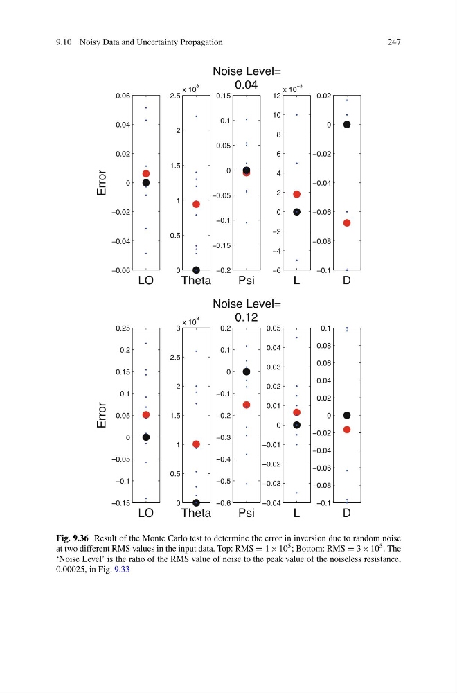
Fig. 9.36 Result of the Monte Carlo test to determine the error in inversion due to random noise
at two different RMS values in the input data. Top: RMS = 1 × 10 5 ; Bottom: RMS = 3 × 10 5 . The
‘Noise Level’ is the ratio of the RMS value of noise to the peak value of the noiseless resistance,
0.00025, in Fig. 9.33
247
−0.06
−0.04
−0.02
0
0.02
0.04
0.06
Error
LO
0
0.5
1
1.5
2
2.5
x 10
8
Theta
−0.2
−0.15
−0.1
−0.05
0
0.05
0.1
0.15
Noise Level=
0.04
Psi
−6
−4
−2
0
2
4
6
8
10
12
x 10
−3
L
−0.1
−0.08
−0.06
−0.04
−0.02
0
0.02
D
−0.15
−0.1
−0.05
0
0.05
0.1
0.15
0.2
0.25
Error
LO
0
0.5
1
1.5
2
2.5
3
x 10
8
Theta
−0.6
−0.5
−0.4
−0.3
−0.2
−0.1
0
0.1
0.2
Noise Level=
0.12
Psi
−0.04
−0.03
−0.02
−0.01
0
0.01
0.02
0.03
0.04
0.05
L
−0.1
−0.08
−0.06
−0.04
−0.02
0
0.02
0.04
0.06
0.08
0.1
D
Fig. 9.36 Result of the Monte Carlo test to determine the error in inversion due to random noise
at two different RMS values in the input data. Top: RMS = 1 × 10 5 ; Bottom: RMS = 3 × 10 5 . The
‘Noise Level’ is the ratio of the RMS value of noise to the peak value of the noiseless resistance,
0.00025, in Fig. 9.33