

1.3 The Algorithm
13
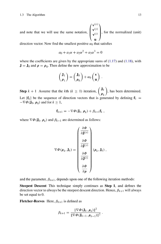
and note that we will use the same notation,
⎛
⎜
⎜
⎝
v (x)
v (y)
v (z)
u
⎞
⎟
⎟
⎠ , for the normalized (unit)
direction vector. Now find the smallest positive α 0 that satisfies
a 0 + a 1 α + a 2 α
2
+ a 3 α
3
= 0
where the coefficients are given by the appropriate sums of (1.17) and (1.18), with
J = J 0 and ρ = ρ 0 . Then define the new approximation to be
J 1
ρ 1
=
J 0
ρ 0
+ α 0
v
u
.
Step k + 1 Assume that the kth (k ≥ 1) iteration,
J k
ρ k
, has been determined.
Let {f k } be the sequence of direction vectors that is generated by defining f 1 =
−∇Φ(J 0 , ρ 0 ) and for k ≥ 1,
f k+1 = −∇Φ(J k , ρ k ) + β k+1 f k ,
where ∇Φ(J k , ρ k ) and β k+1 are determined as follows:
∇Φ(ρ k , J k ) =
⎛
⎜
⎜
⎜
⎜
⎜
⎜
⎜
⎜
⎜
⎜
⎜
⎜
⎜
⎜
⎜
⎝
∂Φ
∂J (x)
∂Φ
∂J (y)
∂Φ
∂J (z)
∂Φ
∂ρ
⎞
⎟
⎟
⎟
⎟
⎟
⎟
⎟
⎟
⎟
⎟
⎟
⎟
⎟
⎟
⎟
⎠
(ρ k , J k ) ,
and the parameter, β k+1 , depends upon one of the following iteration methods:
Steepest Descent This technique simply continues as Step 1, and defines the
direction vector to always be the steepest descent direction. Hence, β k+1 will always
be set equal to 0.
Fletcher-Reeves Here, β k+1 is defined as
β k+1 =
∇Φ(J k , ρ k ) 2
∇Φ(J k−1 , ρ k−1 ) 2 .
13
and note that we will use the same notation,
⎛
⎜
⎜
⎝
v (x)
v (y)
v (z)
u
⎞
⎟
⎟
⎠ , for the normalized (unit)
direction vector. Now find the smallest positive α 0 that satisfies
a 0 + a 1 α + a 2 α
2
+ a 3 α
3
= 0
where the coefficients are given by the appropriate sums of (1.17) and (1.18), with
J = J 0 and ρ = ρ 0 . Then define the new approximation to be
J 1
ρ 1
=
J 0
ρ 0
+ α 0
v
u
.
Step k + 1 Assume that the kth (k ≥ 1) iteration,
J k
ρ k
, has been determined.
Let {f k } be the sequence of direction vectors that is generated by defining f 1 =
−∇Φ(J 0 , ρ 0 ) and for k ≥ 1,
f k+1 = −∇Φ(J k , ρ k ) + β k+1 f k ,
where ∇Φ(J k , ρ k ) and β k+1 are determined as follows:
∇Φ(ρ k , J k ) =
⎛
⎜
⎜
⎜
⎜
⎜
⎜
⎜
⎜
⎜
⎜
⎜
⎜
⎜
⎜
⎜
⎝
∂Φ
∂J (x)
∂Φ
∂J (y)
∂Φ
∂J (z)
∂Φ
∂ρ
⎞
⎟
⎟
⎟
⎟
⎟
⎟
⎟
⎟
⎟
⎟
⎟
⎟
⎟
⎟
⎟
⎠
(ρ k , J k ) ,
and the parameter, β k+1 , depends upon one of the following iteration methods:
Steepest Descent This technique simply continues as Step 1, and defines the
direction vector to always be the steepest descent direction. Hence, β k+1 will always
be set equal to 0.
Fletcher-Reeves Here, β k+1 is defined as
β k+1 =
∇Φ(J k , ρ k ) 2
∇Φ(J k−1 , ρ k−1 ) 2 .