

14
1 A Bilinear Conjugate-Gradient Inversion Algorithm
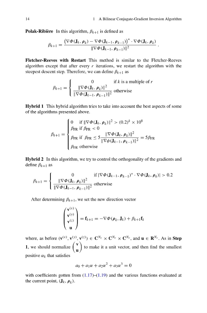
Polak-Ribière In this algorithm, β k+1 is defined as
β k+1 =
∇Φ(J k , ρ k ) − ∇Φ(J k−1 , ρ k−1 )
∗ · ∇Φ(J k , ρ k )
∇Φ(J k−1 , ρ k−1 ) 2
.
Fletcher-Reeves with Restart This method is similar to the Fletcher-Reeves
algorithm except that after every r iterations, we restart the algorithm with the
steepest descent step. Therefore, we can define β k+1 as
β k+1 =
⎧
⎨
⎩
0
i fk is a multiple of r
∇Φ(J k , ρ k ) 2
∇Φ(J k−1 , ρ k−1 ) 2 otherwise
Hybrid 1 This hybrid algorithm tries to take into account the best aspects of some
of the algorithms presented above.
β k+1 =
⎧
⎪ ⎪ ⎪ ⎪ ⎪ ⎨
⎪ ⎪ ⎪ ⎪ ⎪ ⎩
0 if ∇Φ(J k , ρ k ) 2 > (0.2) k × 10 8
β FR if β PR < 0
β PR if β PR ≤ 5
∇Φ(J k , ρ k ) 2
∇φ(J k−1 , ρ k−1 ) 2 = 5β FR
β FR otherwise
Hybrid 2 In this algorithm, we try to control the orthogonality of the gradients and
define β k+1 as
β k+1 =
⎧
⎨
⎩
0
i f|∇Φ(J k−1 , ρ k−1 ) ∗ · ∇Φ(J k , ρ k )| > 0.2
∇Φ(J k , ρ k ) 2
∇Φ(J k−1 , ρ k−1 ) 2 otherwise
After determining β k+1 , we set the new direction vector
⎛
⎜
⎜
⎝
v (x)
v (y)
v (z)
u
⎞
⎟
⎟
⎠ = f k+1 = −∇Φ(ρ k , J k ) + β k+1 f k
where, as before (v (x) , v (y) , v (z) ) ∈ C N c × C N c × C N c , and u ∈ R N c . As in Step
1, we should normalize
v
u
to make it a unit vector, and then find the smallest
positive α k that satisfies
a 0 + a 1 α + a 2 α
2
+ a 3 α
3
= 0
with coefficients gotten from (1.17)–(1.19) and the various functions evaluated at
the current point, (J k , ρ k ).
1 A Bilinear Conjugate-Gradient Inversion Algorithm
Polak-Ribière In this algorithm, β k+1 is defined as
β k+1 =
∇Φ(J k , ρ k ) − ∇Φ(J k−1 , ρ k−1 )
∗ · ∇Φ(J k , ρ k )
∇Φ(J k−1 , ρ k−1 ) 2
.
Fletcher-Reeves with Restart This method is similar to the Fletcher-Reeves
algorithm except that after every r iterations, we restart the algorithm with the
steepest descent step. Therefore, we can define β k+1 as
β k+1 =
⎧
⎨
⎩
0
i fk is a multiple of r
∇Φ(J k , ρ k ) 2
∇Φ(J k−1 , ρ k−1 ) 2 otherwise
Hybrid 1 This hybrid algorithm tries to take into account the best aspects of some
of the algorithms presented above.
β k+1 =
⎧
⎪ ⎪ ⎪ ⎪ ⎪ ⎨
⎪ ⎪ ⎪ ⎪ ⎪ ⎩
0 if ∇Φ(J k , ρ k ) 2 > (0.2) k × 10 8
β FR if β PR < 0
β PR if β PR ≤ 5
∇Φ(J k , ρ k ) 2
∇φ(J k−1 , ρ k−1 ) 2 = 5β FR
β FR otherwise
Hybrid 2 In this algorithm, we try to control the orthogonality of the gradients and
define β k+1 as
β k+1 =
⎧
⎨
⎩
0
i f|∇Φ(J k−1 , ρ k−1 ) ∗ · ∇Φ(J k , ρ k )| > 0.2
∇Φ(J k , ρ k ) 2
∇Φ(J k−1 , ρ k−1 ) 2 otherwise
After determining β k+1 , we set the new direction vector
⎛
⎜
⎜
⎝
v (x)
v (y)
v (z)
u
⎞
⎟
⎟
⎠ = f k+1 = −∇Φ(ρ k , J k ) + β k+1 f k
where, as before (v (x) , v (y) , v (z) ) ∈ C N c × C N c × C N c , and u ∈ R N c . As in Step
1, we should normalize
v
u
to make it a unit vector, and then find the smallest
positive α k that satisfies
a 0 + a 1 α + a 2 α
2
+ a 3 α
3
= 0
with coefficients gotten from (1.17)–(1.19) and the various functions evaluated at
the current point, (J k , ρ k ).