

12
1 A Bilinear Conjugate-Gradient Inversion Algorithm
1.3 The Algorithm
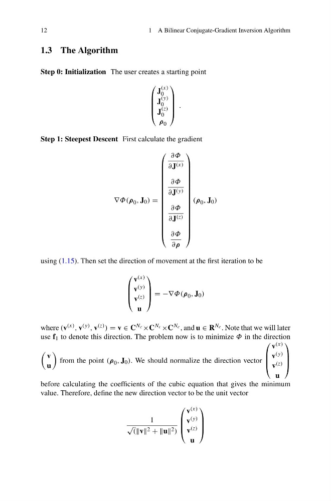
Step 0: Initialization The user creates a starting point
⎛
⎜
⎜
⎜
⎝
J
(x)
0
J
(y)
0
J
(z)
0
ρ 0
⎞
⎟
⎟
⎟
⎠
.
Step 1: Steepest Descent First calculate the gradient
∇Φ(ρ 0 , J 0 ) =
⎛
⎜
⎜
⎜
⎜
⎜
⎜
⎜
⎜
⎜
⎜
⎜
⎜
⎜
⎜
⎜
⎝
∂Φ
∂J (x)
∂Φ
∂J (y)
∂Φ
∂J (z)
∂Φ
∂ρ
⎞
⎟
⎟
⎟
⎟
⎟
⎟
⎟
⎟
⎟
⎟
⎟
⎟
⎟
⎟
⎟
⎠
(ρ 0 , J 0 )
using (1.15). Then set the direction of movement at the first iteration to be
⎛
⎜
⎜
⎝
v (x)
v (y)
v (z)
u
⎞
⎟
⎟
⎠ = −∇Φ(ρ 0 , J 0 )
where (v (x) , v (y) , v (z) ) = v ∈ C N c ×C N c ×C N c , and u ∈ R N c . Note that we will later
use f 1 to denote this direction. The problem now is to minimize Φ in the direction
v
u
from the point (ρ 0 , J 0 ). We should normalize the direction vector
⎛
⎜
⎜
⎝
v (x)
v (y)
v (z)
u
⎞
⎟
⎟
⎠
before calculating the coefficients of the cubic equation that gives the minimum
value. Therefore, define the new direction vector to be the unit vector
1
√
(v 2 + +u 2 )
⎛
⎜
⎜
⎝
v (x)
v (y)
v (z)
u
⎞
⎟
⎟
⎠
1 A Bilinear Conjugate-Gradient Inversion Algorithm
1.3 The Algorithm
Step 0: Initialization The user creates a starting point
⎛
⎜
⎜
⎜
⎝
J
(x)
0
J
(y)
0
J
(z)
0
ρ 0
⎞
⎟
⎟
⎟
⎠
.
Step 1: Steepest Descent First calculate the gradient
∇Φ(ρ 0 , J 0 ) =
⎛
⎜
⎜
⎜
⎜
⎜
⎜
⎜
⎜
⎜
⎜
⎜
⎜
⎜
⎜
⎜
⎝
∂Φ
∂J (x)
∂Φ
∂J (y)
∂Φ
∂J (z)
∂Φ
∂ρ
⎞
⎟
⎟
⎟
⎟
⎟
⎟
⎟
⎟
⎟
⎟
⎟
⎟
⎟
⎟
⎟
⎠
(ρ 0 , J 0 )
using (1.15). Then set the direction of movement at the first iteration to be
⎛
⎜
⎜
⎝
v (x)
v (y)
v (z)
u
⎞
⎟
⎟
⎠ = −∇Φ(ρ 0 , J 0 )
where (v (x) , v (y) , v (z) ) = v ∈ C N c ×C N c ×C N c , and u ∈ R N c . Note that we will later
use f 1 to denote this direction. The problem now is to minimize Φ in the direction
v
u
from the point (ρ 0 , J 0 ). We should normalize the direction vector
⎛
⎜
⎜
⎝
v (x)
v (y)
v (z)
u
⎞
⎟
⎟
⎠
before calculating the coefficients of the cubic equation that gives the minimum
value. Therefore, define the new direction vector to be the unit vector
1
√
(v 2 + +u 2 )
⎛
⎜
⎜
⎝
v (x)
v (y)
v (z)
u
⎞
⎟
⎟
⎠