

1.2 A Bilinear Conjugate-Gradient Inversion Algorithm Using Volume-Integrals
11
B 2x = Q
(x) (u) · v
(x)
A
∗
0y = J
(y)∗
· Q
(y)T (u) + v
(y)∗
· Q
(y)T (ρ) + v
(x)∗
· G
(yx)H
+v
(y)∗
· G
(yy)H
+ v
(z)∗
· G
(yz)H
A
∗
1y = 2v
(y)∗
· Q
(y)T (u)
B 0y = Q
(y) (ρ) · J
(y)
+ G
(yx)
· J
(x)
+G
(yy)
· J
(y)
+ G
(yz)
· J
(z)
− E
(0y)
B 1y = Q
(y) (u) · J
(y)
+ Q
(y) (ρ) · v
(y)
+ G
(yx)
· v
(x)
+G
(yy)
· v
(y)
+ G
(yz)
· v
(z)
B 2y = Q
(y) (u) · v
(y)
A
∗
0z = J
(z)∗
· Q
(z)T (u) + v
(z)∗
· Q
(z)T (ρ) + v
(x)∗
· G
(zx)H
+v
(y)∗
· G
(zy)H
+ v
(z)∗
· G
(zz)H
A
∗
1z = 2v
(z)∗
· Q
(z)T (u)
B 0z = Q
(z) (ρ) · J
(z)
+ G
(zx)
· J
(x)
+G
(zy)
· J
(y)
+ G
(zz)
· J
(z)
− E
(0z)
B 1z = Q
(z) (u) · J
(z)
+ Q
(z) (ρ) · v
(z)
+ G
(zx)
· v
(x)
+G
(zy)
· v
(y)
+ G
(zz)
· v
(z)
B 2z = Q
(z) (u) · v
(z) ,
(1.19)
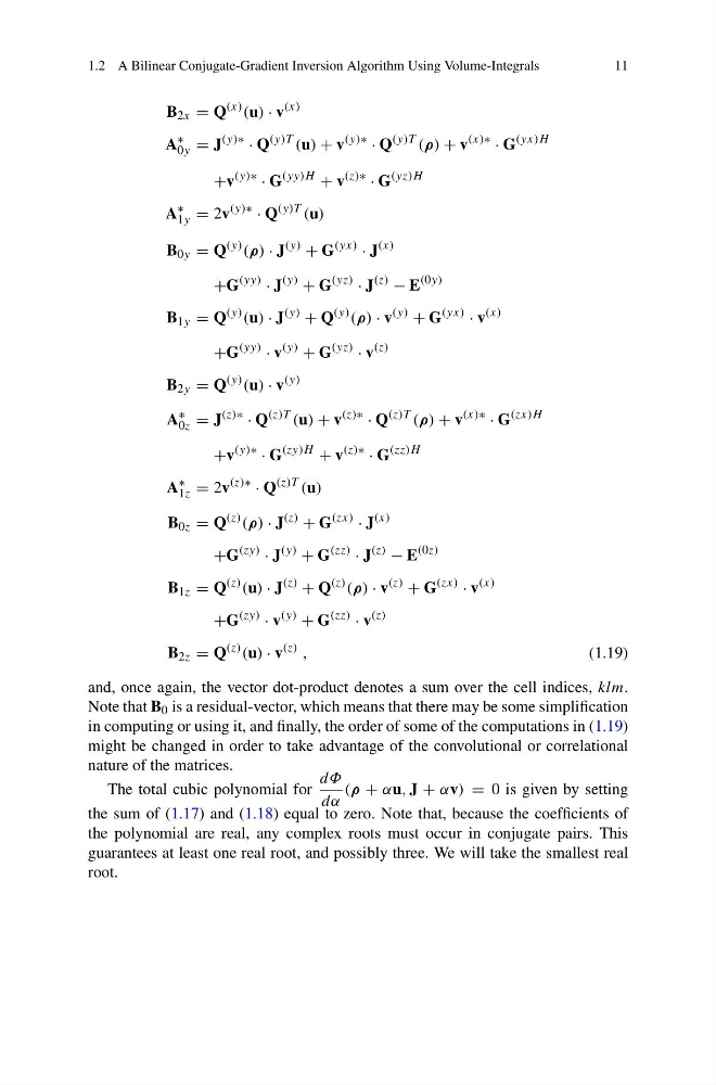
and, once again, the vector dot-product denotes a sum over the cell indices, klm.
Note that B 0 is a residual-vector, which means that there may be some simplification
in computing or using it, and finally, the order of some of the computations in (1.19)
might be changed in order to take advantage of the convolutional or correlational
nature of the matrices.
The total cubic polynomial for
dΦ
dα
(ρ + αu, J + αv) = 0 is given by setting
the sum of (1.17) and (1.18) equal to zero. Note that, because the coefficients of
the polynomial are real, any complex roots must occur in conjugate pairs. This
guarantees at least one real root, and possibly three. We will take the smallest real
root.
11
B 2x = Q
(x) (u) · v
(x)
A
∗
0y = J
(y)∗
· Q
(y)T (u) + v
(y)∗
· Q
(y)T (ρ) + v
(x)∗
· G
(yx)H
+v
(y)∗
· G
(yy)H
+ v
(z)∗
· G
(yz)H
A
∗
1y = 2v
(y)∗
· Q
(y)T (u)
B 0y = Q
(y) (ρ) · J
(y)
+ G
(yx)
· J
(x)
+G
(yy)
· J
(y)
+ G
(yz)
· J
(z)
− E
(0y)
B 1y = Q
(y) (u) · J
(y)
+ Q
(y) (ρ) · v
(y)
+ G
(yx)
· v
(x)
+G
(yy)
· v
(y)
+ G
(yz)
· v
(z)
B 2y = Q
(y) (u) · v
(y)
A
∗
0z = J
(z)∗
· Q
(z)T (u) + v
(z)∗
· Q
(z)T (ρ) + v
(x)∗
· G
(zx)H
+v
(y)∗
· G
(zy)H
+ v
(z)∗
· G
(zz)H
A
∗
1z = 2v
(z)∗
· Q
(z)T (u)
B 0z = Q
(z) (ρ) · J
(z)
+ G
(zx)
· J
(x)
+G
(zy)
· J
(y)
+ G
(zz)
· J
(z)
− E
(0z)
B 1z = Q
(z) (u) · J
(z)
+ Q
(z) (ρ) · v
(z)
+ G
(zx)
· v
(x)
+G
(zy)
· v
(y)
+ G
(zz)
· v
(z)
B 2z = Q
(z) (u) · v
(z) ,
(1.19)
and, once again, the vector dot-product denotes a sum over the cell indices, klm.
Note that B 0 is a residual-vector, which means that there may be some simplification
in computing or using it, and finally, the order of some of the computations in (1.19)
might be changed in order to take advantage of the convolutional or correlational
nature of the matrices.
The total cubic polynomial for
dΦ
dα
(ρ + αu, J + αv) = 0 is given by setting
the sum of (1.17) and (1.18) equal to zero. Note that, because the coefficients of
the polynomial are real, any complex roots must occur in conjugate pairs. This
guarantees at least one real root, and possibly three. We will take the smallest real
root.