

230
9 High-Dimension Model Representation via Sparse GridTechniques
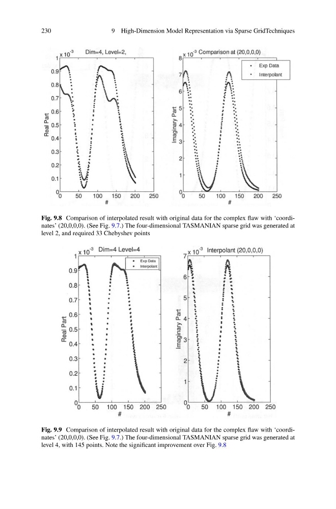
Fig. 9.8 Comparison of interpolated result with original data for the complex flaw with ‘coordinates’ (20,0,0,0). (See Fig. 9.7.) The four-dimensional TASMANIAN sparse grid was generated at
level 2, and required 33 Chebyshev points
Fig. 9.9 Comparison of interpolated result with original data for the complex flaw with ‘coordinates’ (20,0,0,0). (See Fig. 9.7.) The four-dimensional TASMANIAN sparse grid was generated at
level 4, with 145 points. Note the significant improvement over Fig. 9.8
9 High-Dimension Model Representation via Sparse GridTechniques
Fig. 9.8 Comparison of interpolated result with original data for the complex flaw with ‘coordinates’ (20,0,0,0). (See Fig. 9.7.) The four-dimensional TASMANIAN sparse grid was generated at
level 2, and required 33 Chebyshev points
Fig. 9.9 Comparison of interpolated result with original data for the complex flaw with ‘coordinates’ (20,0,0,0). (See Fig. 9.7.) The four-dimensional TASMANIAN sparse grid was generated at
level 4, with 145 points. Note the significant improvement over Fig. 9.8