

9.6 Results for 4D-Level 8
229
with x i
1 = 0 if m i = 1. In order for the knots to be nested at the next level of
approximation, we choose m 1 = 1 and m i = 2 i−1 + 1 for i > 1 [15]. The Lagrange
interpolator is an example of Eq. (1.3) in the TASMANIAN User Manual.
9.5 First TASMANIAN Results
In order to test the accuracy of interpolating high-dimensional models at various
levels, 1 we start with a simple example in which we compare the interpolated result
at various levels with original data that are computed directly with VIC-3D ® for
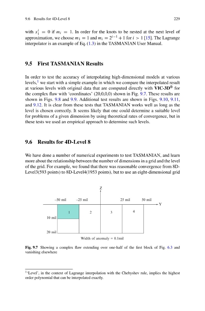
the complex flaw with ‘coordinates’ (20,0,0,0) shown in Fig. 9.7. These results are
shown in Figs. 9.8 and 9.9. Additional test results are shown in Figs. 9.10, 9.11,
and 9.12. It is clear from these tests that TASMANIAN works well as long as the
level is chosen correctly. It seems likely that one could determine a suitable level
for problems of a given dimension by using theoretical rates of convergence, but in
these tests we used an empirical approach to determine such levels.
9.6 Results for 4D-Level 8
We have done a number of numerical experiments to test TASMANIAN, and learn
more about the relationship between the number of dimensions in a grid and the level
of the grid. For example, we found that there was reasonable convergence from 8DLevel3(593 points) to 8D-Level4(1953 points), but to use an eight-dimensional grid
1
4
2
3
Y
Z
20 mil
–25 mil
50 mil
25 mil
Width of anomaly = 0.1mil
–50 mil
10 mil
Fig. 9.7 Showing a complex flaw extending over one-half of the first block of Fig. 6.3 and
vanishing elsewhere
1 ‘Level’, in the context of Lagrange interpolation with the Chebyshev rule, implies the highest
order polynomial that can be interpolated exactly.
229
with x i
1 = 0 if m i = 1. In order for the knots to be nested at the next level of
approximation, we choose m 1 = 1 and m i = 2 i−1 + 1 for i > 1 [15]. The Lagrange
interpolator is an example of Eq. (1.3) in the TASMANIAN User Manual.
9.5 First TASMANIAN Results
In order to test the accuracy of interpolating high-dimensional models at various
levels, 1 we start with a simple example in which we compare the interpolated result
at various levels with original data that are computed directly with VIC-3D ® for
the complex flaw with ‘coordinates’ (20,0,0,0) shown in Fig. 9.7. These results are
shown in Figs. 9.8 and 9.9. Additional test results are shown in Figs. 9.10, 9.11,
and 9.12. It is clear from these tests that TASMANIAN works well as long as the
level is chosen correctly. It seems likely that one could determine a suitable level
for problems of a given dimension by using theoretical rates of convergence, but in
these tests we used an empirical approach to determine such levels.
9.6 Results for 4D-Level 8
We have done a number of numerical experiments to test TASMANIAN, and learn
more about the relationship between the number of dimensions in a grid and the level
of the grid. For example, we found that there was reasonable convergence from 8DLevel3(593 points) to 8D-Level4(1953 points), but to use an eight-dimensional grid
1
4
2
3
Y
Z
20 mil
–25 mil
50 mil
25 mil
Width of anomaly = 0.1mil
–50 mil
10 mil
Fig. 9.7 Showing a complex flaw extending over one-half of the first block of Fig. 6.3 and
vanishing elsewhere
1 ‘Level’, in the context of Lagrange interpolation with the Chebyshev rule, implies the highest
order polynomial that can be interpolated exactly.