

224
9 High-Dimension Model Representation via Sparse GridTechniques
0
1
0.5
0.5
1
0
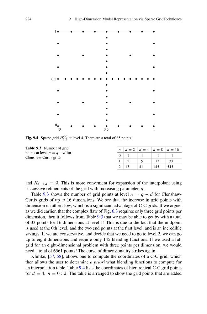
Fig. 9.4 Sparse grid H CC
6,2 at level 4. There are a total of 65 points
Table 9.3 Number of grid
points at level n = q − d for
Clenshaw-Curtis grids
n d = 2 d = 4 d = 8 d = 16
0
1
1
1
1
1
5
9
17
33
2 13
41
145
545
and H d−1,d = ∅. This is more convenient for expansion of the interpolant using
successive refinements of the grid with increasing parameter, q.
Table 9.3 shows the number of grid points at level n = q − d for ClenshawCurtis grids of up to 16 dimensions. We see that the increase in grid points with
dimension is rather slow, which is a significant advantage of C-C grids. If we argue,
as we did earlier, that the complex flaw of Fig. 6.3 requires only three grid points per
dimension, then it follows from Table 9.3 that we may be able to get by with a total
of 33 points for 16 dimensions at level 1! This is due to the fact that the midpoint
is used at the 0th level, and the two end points at the first level, and is an incredible
savings. If we are conservative, and decide that we need to go to level 2, we can go
up to eight dimensions and require only 145 blending functions. If we used a full
grid for an eight-dimensional problem with three points per dimension, we would
need a total of 6561 points! The curse of dimensionality strikes again.
Klimke, [57, 58], allows one to compute the coordinates of a C-C grid, which
then allows the user to determine a priori what blending functions to compute for
an interpolation table. Table 9.4 lists the coordinates of hierarchical C-C grid points
for d = 4, n = 0 : 2. The table is arranged to show the grid points that are added
9 High-Dimension Model Representation via Sparse GridTechniques
0
1
0.5
0.5
1
0
Fig. 9.4 Sparse grid H CC
6,2 at level 4. There are a total of 65 points
Table 9.3 Number of grid
points at level n = q − d for
Clenshaw-Curtis grids
n d = 2 d = 4 d = 8 d = 16
0
1
1
1
1
1
5
9
17
33
2 13
41
145
545
and H d−1,d = ∅. This is more convenient for expansion of the interpolant using
successive refinements of the grid with increasing parameter, q.
Table 9.3 shows the number of grid points at level n = q − d for ClenshawCurtis grids of up to 16 dimensions. We see that the increase in grid points with
dimension is rather slow, which is a significant advantage of C-C grids. If we argue,
as we did earlier, that the complex flaw of Fig. 6.3 requires only three grid points per
dimension, then it follows from Table 9.3 that we may be able to get by with a total
of 33 points for 16 dimensions at level 1! This is due to the fact that the midpoint
is used at the 0th level, and the two end points at the first level, and is an incredible
savings. If we are conservative, and decide that we need to go to level 2, we can go
up to eight dimensions and require only 145 blending functions. If we used a full
grid for an eight-dimensional problem with three points per dimension, we would
need a total of 6561 points! The curse of dimensionality strikes again.
Klimke, [57, 58], allows one to compute the coordinates of a C-C grid, which
then allows the user to determine a priori what blending functions to compute for
an interpolation table. Table 9.4 lists the coordinates of hierarchical C-C grid points
for d = 4, n = 0 : 2. The table is arranged to show the grid points that are added