

9.3 Clenshaw-Curtis Grids
223
0
1
1
0.5
0
0.5
0
0.5
1
0
0.5
1
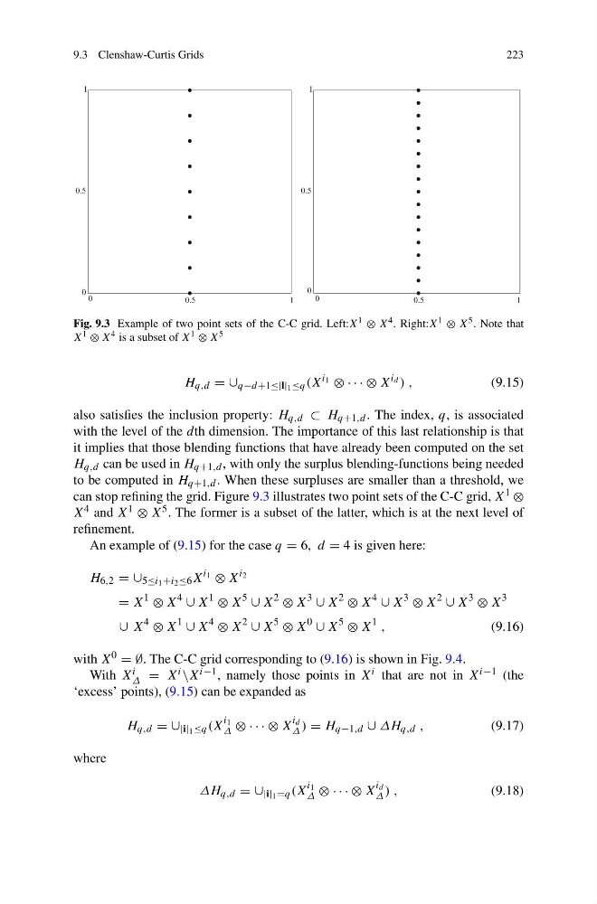
Fig. 9.3 Example of two point sets of the C-C grid. Left:X 1 ⊗ X 4 . Right:X 1 ⊗ X 5 . Note that
X 1 ⊗ X 4 is a subset of X 1 ⊗ X 5
H q,d = ∪ q−d+1≤|l| 1 ≤q (X
i 1 ⊗ · · · ⊗ X
i d ) ,
(9.15)
also satisfies the inclusion property: H q,d ⊂ H q+1,d . The index, q, is associated
with the level of the dth dimension. The importance of this last relationship is that
it implies that those blending functions that have already been computed on the set
H q,d can be used in H q+1,d , with only the surplus blending-functions being needed
to be computed in H q+1,d . When these surpluses are smaller than a threshold, we
can stop refining the grid. Figure 9.3 illustrates two point sets of the C-C grid, X 1 ⊗
X 4 and X 1 ⊗ X 5 . The former is a subset of the latter, which is at the next level of
refinement.
An example of (9.15) for the case q = 6, d = 4 is given here:
H 6,2 = ∪ 5≤i 1 +i 2 ≤6 X
i 1 ⊗ X
i 2
= X
1
⊗ X
4
∪ X
1
⊗ X
5
∪ X
2
⊗ X
3
∪ X
2
⊗ X
4
∪ X
3
⊗ X
2
∪ X
3
⊗ X
3
∪ X
4
⊗ X
1
∪ X
4
⊗ X
2
∪ X
5
⊗ X
0
∪ X
5
⊗ X
1 ,
(9.16)
with X 0 = ∅. The C-C grid corresponding to (9.16) is shown in Fig. 9.4.
With X i
Δ = X i \X i−1 , namely those points in X i that are not in X i−1 (the
‘excess’ points), (9.15) can be expanded as
H q,d = ∪ |i| 1 ≤q (X
i 1
Δ ⊗ · · · ⊗ X
i d
Δ ) = H q−1,d ∪ ΔH q,d ,
(9.17)
where
ΔH q,d = ∪ |i| 1 =q (X
i 1
Δ ⊗ · · · ⊗ X
i d
Δ ) ,
(9.18)
223
0
1
1
0.5
0
0.5
0
0.5
1
0
0.5
1
Fig. 9.3 Example of two point sets of the C-C grid. Left:X 1 ⊗ X 4 . Right:X 1 ⊗ X 5 . Note that
X 1 ⊗ X 4 is a subset of X 1 ⊗ X 5
H q,d = ∪ q−d+1≤|l| 1 ≤q (X
i 1 ⊗ · · · ⊗ X
i d ) ,
(9.15)
also satisfies the inclusion property: H q,d ⊂ H q+1,d . The index, q, is associated
with the level of the dth dimension. The importance of this last relationship is that
it implies that those blending functions that have already been computed on the set
H q,d can be used in H q+1,d , with only the surplus blending-functions being needed
to be computed in H q+1,d . When these surpluses are smaller than a threshold, we
can stop refining the grid. Figure 9.3 illustrates two point sets of the C-C grid, X 1 ⊗
X 4 and X 1 ⊗ X 5 . The former is a subset of the latter, which is at the next level of
refinement.
An example of (9.15) for the case q = 6, d = 4 is given here:
H 6,2 = ∪ 5≤i 1 +i 2 ≤6 X
i 1 ⊗ X
i 2
= X
1
⊗ X
4
∪ X
1
⊗ X
5
∪ X
2
⊗ X
3
∪ X
2
⊗ X
4
∪ X
3
⊗ X
2
∪ X
3
⊗ X
3
∪ X
4
⊗ X
1
∪ X
4
⊗ X
2
∪ X
5
⊗ X
0
∪ X
5
⊗ X
1 ,
(9.16)
with X 0 = ∅. The C-C grid corresponding to (9.16) is shown in Fig. 9.4.
With X i
Δ = X i \X i−1 , namely those points in X i that are not in X i−1 (the
‘excess’ points), (9.15) can be expanded as
H q,d = ∪ |i| 1 ≤q (X
i 1
Δ ⊗ · · · ⊗ X
i d
Δ ) = H q−1,d ∪ ΔH q,d ,
(9.17)
where
ΔH q,d = ∪ |i| 1 =q (X
i 1
Δ ⊗ · · · ⊗ X
i d
Δ ) ,
(9.18)