

9.3 Clenshaw-Curtis Grids
225
x 3,1
x
x
x
x
0
3,1
φ
φ
φ
φ
φ
3,2
3,3
3,4
3,5
3,2
3,3
3,4
3,5
1
1
x
x
x
0
1
1
φ 1,1
2,1
φ
φ 2,2
φ 3,1
3,2
φ
x 2,1
x 3,1
1,1
3,2
2,2
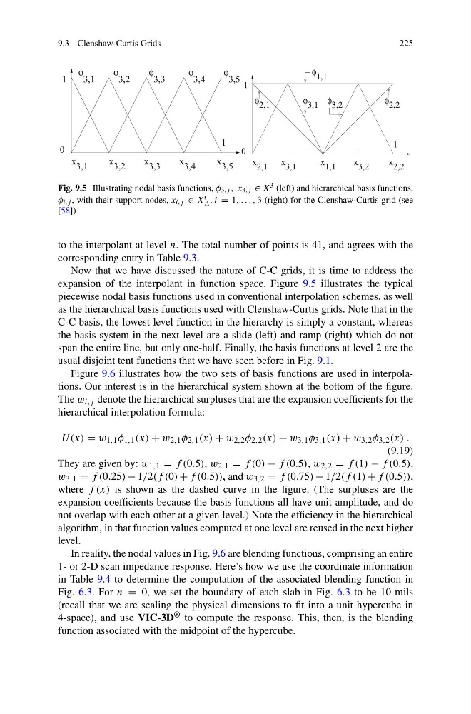
Fig. 9.5 Illustrating nodal basis functions, φ 3,j , x 3,j ∈ X 3 (left) and hierarchical basis functions,
φ i,j , with their support nodes, x i,j ∈ X i
Δ , i = 1, . . . , 3 (right) for the Clenshaw-Curtis grid (see
[58])
to the interpolant at level n. The total number of points is 41, and agrees with the
corresponding entry in Table 9.3.
Now that we have discussed the nature of C-C grids, it is time to address the
expansion of the interpolant in function space. Figure 9.5 illustrates the typical
piecewise nodal basis functions used in conventional interpolation schemes, as well
as the hierarchical basis functions used with Clenshaw-Curtis grids. Note that in the
C-C basis, the lowest level function in the hierarchy is simply a constant, whereas
the basis system in the next level are a slide (left) and ramp (right) which do not
span the entire line, but only one-half. Finally, the basis functions at level 2 are the
usual disjoint tent functions that we have seen before in Fig. 9.1.
Figure 9.6 illustrates how the two sets of basis functions are used in interpolations. Our interest is in the hierarchical system shown at the bottom of the figure.
The w i,j denote the hierarchical surpluses that are the expansion coefficients for the
hierarchical interpolation formula:
U(x) = w 1,1 φ 1,1 (x) + w 2,1 φ 2,1 (x) + w 2,2 φ 2,2 (x) + w 3,1 φ 3,1 (x) + w 3,2 φ 3,2 (x) .
(9.19)
They are given by: w 1,1 = f (0.5), w 2,1 = f (0) − f (0.5), w 2,2 = f (1) − f (0.5),
w 3,1 = f (0.25) − 1/2(f (0) + f (0.5)), and w 3,2 = f (0.75) − 1/2(f (1) + f (0.5)),
where f (x) is shown as the dashed curve in the figure. (The surpluses are the
expansion coefficients because the basis functions all have unit amplitude, and do
not overlap with each other at a given level.) Note the efficiency in the hierarchical
algorithm, in that function values computed at one level are reused in the next higher
level.
In reality, the nodal values in Fig. 9.6 are blending functions, comprising an entire
1- or 2-D scan impedance response. Here’s how we use the coordinate information
in Table 9.4 to determine the computation of the associated blending function in
Fig. 6.3. For n = 0, we set the boundary of each slab in Fig. 6.3 to be 10 mils
(recall that we are scaling the physical dimensions to fit into a unit hypercube in
4-space), and use VIC-3D ® to compute the response. This, then, is the blending
function associated with the midpoint of the hypercube.
225
x 3,1
x
x
x
x
0
3,1
φ
φ
φ
φ
φ
3,2
3,3
3,4
3,5
3,2
3,3
3,4
3,5
1
1
x
x
x
0
1
1
φ 1,1
2,1
φ
φ 2,2
φ 3,1
3,2
φ
x 2,1
x 3,1
1,1
3,2
2,2
Fig. 9.5 Illustrating nodal basis functions, φ 3,j , x 3,j ∈ X 3 (left) and hierarchical basis functions,
φ i,j , with their support nodes, x i,j ∈ X i
Δ , i = 1, . . . , 3 (right) for the Clenshaw-Curtis grid (see
[58])
to the interpolant at level n. The total number of points is 41, and agrees with the
corresponding entry in Table 9.3.
Now that we have discussed the nature of C-C grids, it is time to address the
expansion of the interpolant in function space. Figure 9.5 illustrates the typical
piecewise nodal basis functions used in conventional interpolation schemes, as well
as the hierarchical basis functions used with Clenshaw-Curtis grids. Note that in the
C-C basis, the lowest level function in the hierarchy is simply a constant, whereas
the basis system in the next level are a slide (left) and ramp (right) which do not
span the entire line, but only one-half. Finally, the basis functions at level 2 are the
usual disjoint tent functions that we have seen before in Fig. 9.1.
Figure 9.6 illustrates how the two sets of basis functions are used in interpolations. Our interest is in the hierarchical system shown at the bottom of the figure.
The w i,j denote the hierarchical surpluses that are the expansion coefficients for the
hierarchical interpolation formula:
U(x) = w 1,1 φ 1,1 (x) + w 2,1 φ 2,1 (x) + w 2,2 φ 2,2 (x) + w 3,1 φ 3,1 (x) + w 3,2 φ 3,2 (x) .
(9.19)
They are given by: w 1,1 = f (0.5), w 2,1 = f (0) − f (0.5), w 2,2 = f (1) − f (0.5),
w 3,1 = f (0.25) − 1/2(f (0) + f (0.5)), and w 3,2 = f (0.75) − 1/2(f (1) + f (0.5)),
where f (x) is shown as the dashed curve in the figure. (The surpluses are the
expansion coefficients because the basis functions all have unit amplitude, and do
not overlap with each other at a given level.) Note the efficiency in the hierarchical
algorithm, in that function values computed at one level are reused in the next higher
level.
In reality, the nodal values in Fig. 9.6 are blending functions, comprising an entire
1- or 2-D scan impedance response. Here’s how we use the coordinate information
in Table 9.4 to determine the computation of the associated blending function in
Fig. 6.3. For n = 0, we set the boundary of each slab in Fig. 6.3 to be 10 mils
(recall that we are scaling the physical dimensions to fit into a unit hypercube in
4-space), and use VIC-3D ® to compute the response. This, then, is the blending
function associated with the midpoint of the hypercube.