

8.5 The Geometric Autocorrelation Function
209
HTN1-cleaned 0 - 81 - nodes
1
0.9
0.8
0.7
0.6
0.5
0.4
0.3
0.2
0.1
0
0
500
1000
1500
2000
2500
distance, micrometers
Probability
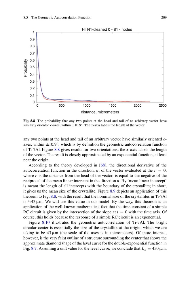
Fig. 8.8 The probability that any two points at the head and tail of an arbitrary vector have
similarly oriented c-axes, within ±10.9 ◦ . The x-axis labels the length of the vector
any two points at the head and tail of an arbitrary vector have similarly oriented caxes, within ±10.9 ◦ , which is by definition the geometric autocorrelation function
of Ti-7Al. Figure 8.8 gives results for two orientations; the x-axis labels the length
of the vector. The result is closely approximated by an exponential function, at least
near the origin.
According to the theory developed in [68], the directional derivative of the
autocorrelation function in the direction, n, of the vector evaluated at the r = 0,
where r is the distance from the head of the vector, is equal to the negative of the
reciprocal of the mean linear intercept in the direction n. By ‘mean linear intercept’
is meant the length of all intercepts with the boundary of the crystallite; in short,
it gives us the mean size of the crystallite. Figure 8.9 depicts an application of this
theorem to Fig. 8.8, with the result that the nominal size of the crystallites in Ti-7Al
is ≈43 µm. We will use this value in our model. By the way, this theorem is an
application of the well-known mathematical fact that the time-constant of a simple
RC circuit is given by the intersection of the slope at t = 0 with the time axis. Of
course, this holds because the response of a simple RC circuit is an exponential.
Figure 8.10 illustrates the geometric autocorrelation of Ti-7Al. The bright
circular center is essentially the size of the crystallite at the origin, which we are
taking to be 43 µm (the scale of the axes is in micrometers). Of more interest,
however, is the very faint outline of a structure surrounding the center that shows the
approximate diamond shape of the level curve for the double-exponential function in
Fig. 8.7. Assuming a unit value for the level curve, we conclude that L x = 430 µm,
209
HTN1-cleaned 0 - 81 - nodes
1
0.9
0.8
0.7
0.6
0.5
0.4
0.3
0.2
0.1
0
0
500
1000
1500
2000
2500
distance, micrometers
Probability
Fig. 8.8 The probability that any two points at the head and tail of an arbitrary vector have
similarly oriented c-axes, within ±10.9 ◦ . The x-axis labels the length of the vector
any two points at the head and tail of an arbitrary vector have similarly oriented caxes, within ±10.9 ◦ , which is by definition the geometric autocorrelation function
of Ti-7Al. Figure 8.8 gives results for two orientations; the x-axis labels the length
of the vector. The result is closely approximated by an exponential function, at least
near the origin.
According to the theory developed in [68], the directional derivative of the
autocorrelation function in the direction, n, of the vector evaluated at the r = 0,
where r is the distance from the head of the vector, is equal to the negative of the
reciprocal of the mean linear intercept in the direction n. By ‘mean linear intercept’
is meant the length of all intercepts with the boundary of the crystallite; in short,
it gives us the mean size of the crystallite. Figure 8.9 depicts an application of this
theorem to Fig. 8.8, with the result that the nominal size of the crystallites in Ti-7Al
is ≈43 µm. We will use this value in our model. By the way, this theorem is an
application of the well-known mathematical fact that the time-constant of a simple
RC circuit is given by the intersection of the slope at t = 0 with the time axis. Of
course, this holds because the response of a simple RC circuit is an exponential.
Figure 8.10 illustrates the geometric autocorrelation of Ti-7Al. The bright
circular center is essentially the size of the crystallite at the origin, which we are
taking to be 43 µm (the scale of the axes is in micrometers). Of more interest,
however, is the very faint outline of a structure surrounding the center that shows the
approximate diamond shape of the level curve for the double-exponential function in
Fig. 8.7. Assuming a unit value for the level curve, we conclude that L x = 430 µm,