

202
8 A Model for Microstructure Characterization
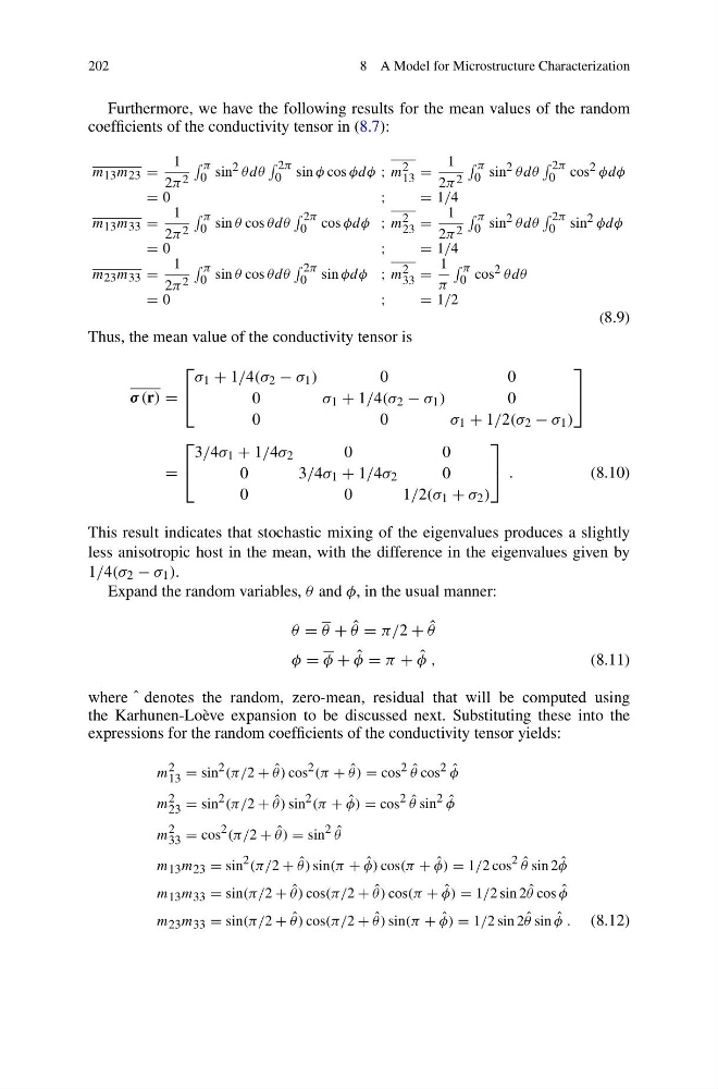
Furthermore, we have the following results for the mean values of the random
coefficients of the conductivity tensor in (8.7):
m 13 m 23 =
1
2π 2
π
0 sin 2 θdθ
2π
0 sin φ cos φdφ ; m 2
13 =
1
2π 2
π
0 sin 2 θdθ
2π
0 cos 2 φdφ
= 0
;
=1/4
m 13 m 33 =
1
2π 2
π
0 sin θ cos θdθ
2π
0 cos φdφ ; m 2
23 =
1
2π 2
π
0 sin 2 θdθ
2π
0 sin 2 φdφ
= 0
;
=1/4
m 23 m 33 =
1
2π 2
π
0 sin θ cos θdθ
2π
0 sin φdφ ; m 2
33 =
1
π
π
0 cos 2 θdθ
= 0
;
=1/2
(8.9)
Thus, the mean value of the conductivity tensor is
σ (r) =
⎡
⎣
σ 1 + 1/4(σ 2 − σ 1 )
0
0
0
σ 1 + 1/4(σ 2 − σ 1 )
0
0
0
σ 1 + 1/2(σ 2 − σ 1 )
⎤
⎦
=
⎡
⎣
3/4σ 1 + 1/4σ 2
0
0
0
3 /4σ 1 + 1/4σ 2
0
0
0
1 /2(σ 1 + σ 2 )
⎤
⎦ .
(8.10)
This result indicates that stochastic mixing of the eigenvalues produces a slightly
less anisotropic host in the mean, with the difference in the eigenvalues given by
1/4(σ 2 − σ 1 ).
Expand the random variables, θ and φ, in the usual manner:
θ = θ + ˆ
θ = π/2 + ˆ
θ
φ = φ + ˆ
φ = π + ˆ
φ ,
(8.11)
where ˆ denotes the random, zero-mean, residual that will be computed using
the Karhunen-Loève expansion to be discussed next. Substituting these into the
expressions for the random coefficients of the conductivity tensor yields:
m 2
13 = sin 2 (π/2 + ˆ
θ) cos 2 (π + ˆ
θ) = cos 2 ˆ
θ cos 2 ˆ
φ
m 2
23 = sin 2 (π/2 + ˆ
θ) sin 2 (π + ˆ
φ) = cos 2 ˆ
θ sin 2 ˆ
φ
m 2
33 = cos 2 (π/2 + ˆ
θ) = sin 2 ˆ
θ
m 13 m 23 = sin 2 (π/2 + ˆ
θ) sin(π + ˆ
φ) cos(π + ˆ
φ) = 1/2 cos 2 ˆ
θ sin 2 ˆ
φ
m 13 m 33 = sin(π/2 + ˆ
θ) cos(π/2 + ˆ
θ) cos(π + ˆ
φ) = 1/2 sin 2 ˆ
θ cos ˆ
φ
m 23 m 33 = sin(π/2 + ˆ
θ) cos(π/2 + ˆ
θ) sin(π + ˆ
φ) = 1/2 sin 2 ˆ
θ sin ˆ
φ . (8.12)
8 A Model for Microstructure Characterization
Furthermore, we have the following results for the mean values of the random
coefficients of the conductivity tensor in (8.7):
m 13 m 23 =
1
2π 2
π
0 sin 2 θdθ
2π
0 sin φ cos φdφ ; m 2
13 =
1
2π 2
π
0 sin 2 θdθ
2π
0 cos 2 φdφ
= 0
;
=1/4
m 13 m 33 =
1
2π 2
π
0 sin θ cos θdθ
2π
0 cos φdφ ; m 2
23 =
1
2π 2
π
0 sin 2 θdθ
2π
0 sin 2 φdφ
= 0
;
=1/4
m 23 m 33 =
1
2π 2
π
0 sin θ cos θdθ
2π
0 sin φdφ ; m 2
33 =
1
π
π
0 cos 2 θdθ
= 0
;
=1/2
(8.9)
Thus, the mean value of the conductivity tensor is
σ (r) =
⎡
⎣
σ 1 + 1/4(σ 2 − σ 1 )
0
0
0
σ 1 + 1/4(σ 2 − σ 1 )
0
0
0
σ 1 + 1/2(σ 2 − σ 1 )
⎤
⎦
=
⎡
⎣
3/4σ 1 + 1/4σ 2
0
0
0
3 /4σ 1 + 1/4σ 2
0
0
0
1 /2(σ 1 + σ 2 )
⎤
⎦ .
(8.10)
This result indicates that stochastic mixing of the eigenvalues produces a slightly
less anisotropic host in the mean, with the difference in the eigenvalues given by
1/4(σ 2 − σ 1 ).
Expand the random variables, θ and φ, in the usual manner:
θ = θ + ˆ
θ = π/2 + ˆ
θ
φ = φ + ˆ
φ = π + ˆ
φ ,
(8.11)
where ˆ denotes the random, zero-mean, residual that will be computed using
the Karhunen-Loève expansion to be discussed next. Substituting these into the
expressions for the random coefficients of the conductivity tensor yields:
m 2
13 = sin 2 (π/2 + ˆ
θ) cos 2 (π + ˆ
θ) = cos 2 ˆ
θ cos 2 ˆ
φ
m 2
23 = sin 2 (π/2 + ˆ
θ) sin 2 (π + ˆ
φ) = cos 2 ˆ
θ sin 2 ˆ
φ
m 2
33 = cos 2 (π/2 + ˆ
θ) = sin 2 ˆ
θ
m 13 m 23 = sin 2 (π/2 + ˆ
θ) sin(π + ˆ
φ) cos(π + ˆ
φ) = 1/2 cos 2 ˆ
θ sin 2 ˆ
φ
m 13 m 33 = sin(π/2 + ˆ
θ) cos(π/2 + ˆ
θ) cos(π + ˆ
φ) = 1/2 sin 2 ˆ
θ cos ˆ
φ
m 23 m 33 = sin(π/2 + ˆ
θ) cos(π/2 + ˆ
θ) sin(π + ˆ
φ) = 1/2 sin 2 ˆ
θ sin ˆ
φ . (8.12)