

8.3 The Karhunen-Loève Model
203
As an aside, we note that if ˆ
θ = ˆ
φ = 0, then (8.12) gives us the values of
the coefficients at the mean of their random arguments, which, as can be seen by
comparison with (8.9), is not equal to the mean of the coefficients. This is due to the
fact that the random coefficients are nonlinear functions of their random arguments.
8.3 The Karhunen-Loève Model
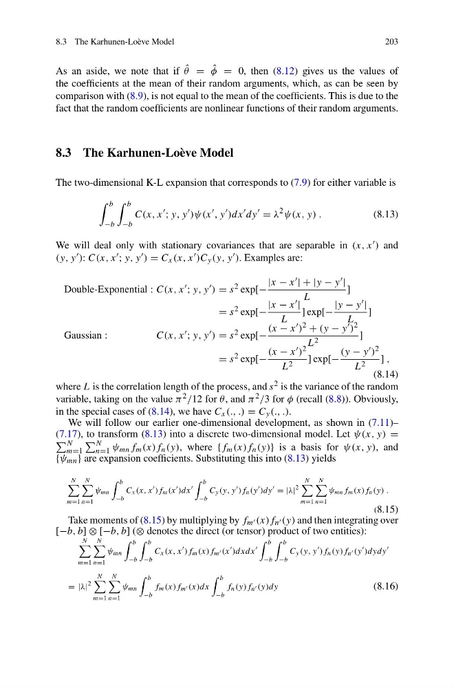
The two-dimensional K-L expansion that corresponds to (7.9) for either variable is
b
−b
b
−b
C(x, x
; y, y
)ψ(x
, y
)dx
dy
= λ
2 ψ(x, y) .
(8.13)
We will deal only with stationary covariances that are separable in (x, x ) and
(y, y ): C(x, x ; y, y ) = C x (x, x )C y (y, y ). Examples are:
Double-Exponential : C(x, x ; y, y ) = s 2 exp[−
|x − x | + |y − y |
L
]
= s 2 exp[−
|x − x |
L
] exp[−
|y − y |
L
]
Gaussian :
C(x, x ; y, y ) = s 2 exp[−
(x − x ) 2 + (y − y ) 2
L 2
]
= s 2 exp[−
(x − x ) 2
L 2 ] exp[−
(y − y ) 2
L 2 ] ,
(8.14)
where L is the correlation length of the process, and s 2 is the variance of the random
variable, taking on the value π 2 /12 for θ , and π 2 /3 for φ (recall (8.8)). Obviously,
in the special cases of (8.14), we have C x (., .) = C y (., .).
We will follow our earlier one-dimensional development, as shown in (7.11)–
(7.17), to transform (8.13) into a discrete two-dimensional model. Let ψ(x, y) =
N
m=1
N
n=1 ψ mn f m (x)f n (y), where {f m (x)f n (y)} is a basis for ψ(x, y), and
{ψ mn } are expansion coefficients. Substituting this into (8.13) yields
N
m=1
N
n=1
ψ mn
b
−b
C x (x, x
)f m (x
)dx
b
−b
C y (y, y
)f n (y
)dy
= |λ|
2
N
m=1
N
n=1
ψ mn f m (x)f n (y) .
(8.15)
Take moments of (8.15) by multiplying by f m (x)f n (y) and then integrating over
[−b, b] ⊗ [−b, b] (⊗ denotes the direct (or tensor) product of two entities):
N
m=1
N
n=1
ψ mn
b
−b
b
−b
C x (x, x
)f m (x)f m (x
)dxdx
b
−b
b
−b
C y (y, y
)f n (y)f n (y
)dydy
= |λ|
2
N
m=1
N
n=1
ψ mn
b
−b
f m (x)f m (x)dx
b
−b
f n (y)f n (y)dy
(8.16)
203
As an aside, we note that if ˆ
θ = ˆ
φ = 0, then (8.12) gives us the values of
the coefficients at the mean of their random arguments, which, as can be seen by
comparison with (8.9), is not equal to the mean of the coefficients. This is due to the
fact that the random coefficients are nonlinear functions of their random arguments.
8.3 The Karhunen-Loève Model
The two-dimensional K-L expansion that corresponds to (7.9) for either variable is
b
−b
b
−b
C(x, x
; y, y
)ψ(x
, y
)dx
dy
= λ
2 ψ(x, y) .
(8.13)
We will deal only with stationary covariances that are separable in (x, x ) and
(y, y ): C(x, x ; y, y ) = C x (x, x )C y (y, y ). Examples are:
Double-Exponential : C(x, x ; y, y ) = s 2 exp[−
|x − x | + |y − y |
L
]
= s 2 exp[−
|x − x |
L
] exp[−
|y − y |
L
]
Gaussian :
C(x, x ; y, y ) = s 2 exp[−
(x − x ) 2 + (y − y ) 2
L 2
]
= s 2 exp[−
(x − x ) 2
L 2 ] exp[−
(y − y ) 2
L 2 ] ,
(8.14)
where L is the correlation length of the process, and s 2 is the variance of the random
variable, taking on the value π 2 /12 for θ , and π 2 /3 for φ (recall (8.8)). Obviously,
in the special cases of (8.14), we have C x (., .) = C y (., .).
We will follow our earlier one-dimensional development, as shown in (7.11)–
(7.17), to transform (8.13) into a discrete two-dimensional model. Let ψ(x, y) =
N
m=1
N
n=1 ψ mn f m (x)f n (y), where {f m (x)f n (y)} is a basis for ψ(x, y), and
{ψ mn } are expansion coefficients. Substituting this into (8.13) yields
N
m=1
N
n=1
ψ mn
b
−b
C x (x, x
)f m (x
)dx
b
−b
C y (y, y
)f n (y
)dy
= |λ|
2
N
m=1
N
n=1
ψ mn f m (x)f n (y) .
(8.15)
Take moments of (8.15) by multiplying by f m (x)f n (y) and then integrating over
[−b, b] ⊗ [−b, b] (⊗ denotes the direct (or tensor) product of two entities):
N
m=1
N
n=1
ψ mn
b
−b
b
−b
C x (x, x
)f m (x)f m (x
)dxdx
b
−b
b
−b
C y (y, y
)f n (y)f n (y
)dydy
= |λ|
2
N
m=1
N
n=1
ψ mn
b
−b
f m (x)f m (x)dx
b
−b
f n (y)f n (y)dy
(8.16)