

8.2 Stochastic Euler Space
201
Data supplied by P. B. Nagy 1 give values of σ 1 = 6.04 × 10 5 S/m (1.04% IACS)
and σ 2 = 5.90 × 10 5 S/m (1.02%IACS) for the basal plane and normal-to-the-basalplane conductivities, respectively.
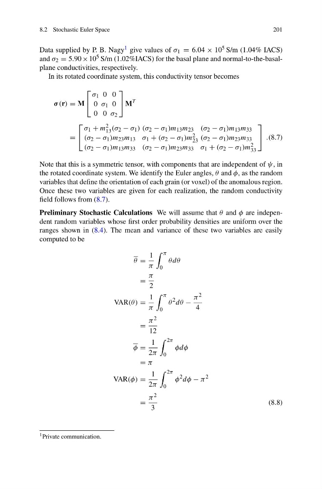
In its rotated coordinate system, this conductivity tensor becomes
σ (r) = M
⎡
⎣
σ 1 0 0
0 σ 1 0
0 0 σ 2
⎤
⎦ M
T
=
⎡
⎣
σ 1 + m 2
13 (σ 2 − σ 1 ) (σ 2 − σ 1 )m 13 m 23 (σ 2 − σ 1 )m 13 m 33
(σ 2 − σ 1 )m 23 m 13 σ 1 + (σ 2 − σ 1 )m 2
23 (σ 2 − σ 1 )m 23 m 33
(σ 2 − σ 1 )m 13 m 33 (σ 2 − σ 1 )m 23 m 33 σ 1 + (σ 2 − σ 1 )m 2
33
⎤
⎦ .(8.7)
Note that this is a symmetric tensor, with components that are independent of ψ, in
the rotated coordinate system. We identify the Euler angles, θ and φ, as the random
variables that define the orientation of each grain (or voxel) of the anomalous region.
Once these two variables are given for each realization, the random conductivity
field follows from (8.7).
Preliminary Stochastic Calculations We will assume that θ and φ are independent random variables whose first order probability densities are uniform over the
ranges shown in (8.4). The mean and variance of these two variables are easily
computed to be
θ =
1
π
π
0
θdθ
=
π
2
VAR(θ ) =
1
π
π
0
θ
2 dθ −
π 2
4
=
π 2
12
φ =
1
2π
2π
0
φdφ
= π
VAR(φ) =
1
2π
2π
0
φ
2 dφ − π
2
=
π 2
3
(8.8)
1 Private communication.
201
Data supplied by P. B. Nagy 1 give values of σ 1 = 6.04 × 10 5 S/m (1.04% IACS)
and σ 2 = 5.90 × 10 5 S/m (1.02%IACS) for the basal plane and normal-to-the-basalplane conductivities, respectively.
In its rotated coordinate system, this conductivity tensor becomes
σ (r) = M
⎡
⎣
σ 1 0 0
0 σ 1 0
0 0 σ 2
⎤
⎦ M
T
=
⎡
⎣
σ 1 + m 2
13 (σ 2 − σ 1 ) (σ 2 − σ 1 )m 13 m 23 (σ 2 − σ 1 )m 13 m 33
(σ 2 − σ 1 )m 23 m 13 σ 1 + (σ 2 − σ 1 )m 2
23 (σ 2 − σ 1 )m 23 m 33
(σ 2 − σ 1 )m 13 m 33 (σ 2 − σ 1 )m 23 m 33 σ 1 + (σ 2 − σ 1 )m 2
33
⎤
⎦ .(8.7)
Note that this is a symmetric tensor, with components that are independent of ψ, in
the rotated coordinate system. We identify the Euler angles, θ and φ, as the random
variables that define the orientation of each grain (or voxel) of the anomalous region.
Once these two variables are given for each realization, the random conductivity
field follows from (8.7).
Preliminary Stochastic Calculations We will assume that θ and φ are independent random variables whose first order probability densities are uniform over the
ranges shown in (8.4). The mean and variance of these two variables are easily
computed to be
θ =
1
π
π
0
θdθ
=
π
2
VAR(θ ) =
1
π
π
0
θ
2 dθ −
π 2
4
=
π 2
12
φ =
1
2π
2π
0
φdφ
= π
VAR(φ) =
1
2π
2π
0
φ
2 dφ − π
2
=
π 2
3
(8.8)
1 Private communication.