

200
8 A Model for Microstructure Characterization
(I 1 , J 1 , K 1 ) → (I 2 , J 2 , k)
⎧
⎨
⎩
I 2 = I 1 cos θ − K 1 sin θ
J 2 = J 1
k = I 1 sin θ + K 1 cos θ
⎫
⎬
⎭
.
(8.2)
Finally, rotate about k to bring I 2 to i and J 2 to j, say through an angle ψ; this
gives the transformation
(I 2 , J 2 , k) → (i, j, k)
⎧
⎨
⎩
i = I 2 cos ψ + J 2 sin ψ
j = −I 2 sin ψ + J 2 cos ψ
k = k
⎫
⎬
⎭
.
(8.3)
The angles (θ, φ, ψ) are the Euler angles. Their values determine the position of
the triad (i, j, k) relative to (I, J, K). The angles range over the following values:
0 ≤ θ ≤ π
0 ≤ φ < 2π
0 ≤ ψ < 2π
.
(8.4)
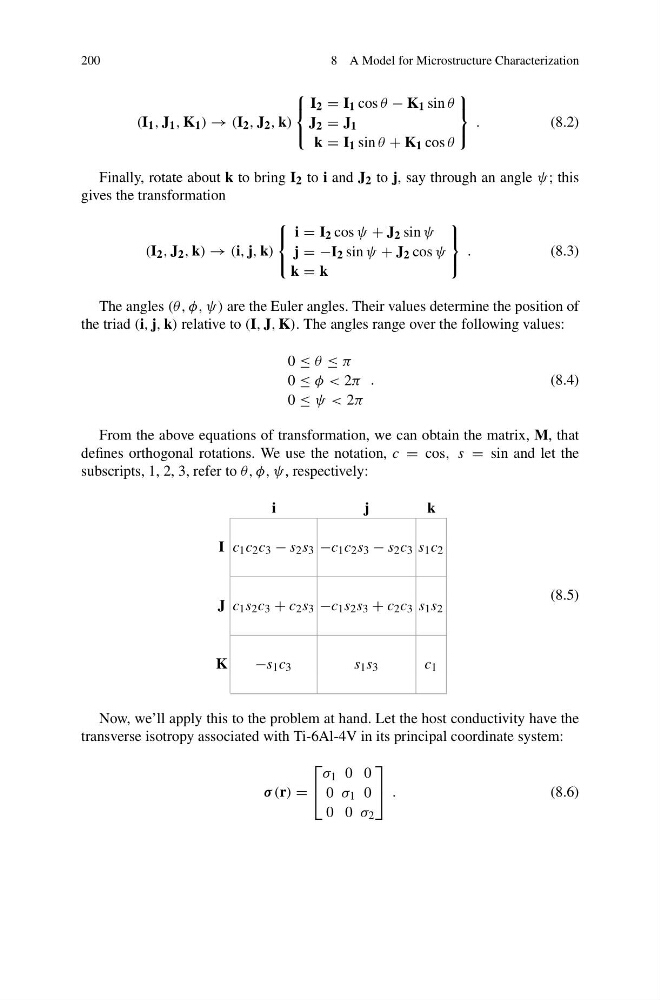
From the above equations of transformation, we can obtain the matrix, M, that
defines orthogonal rotations. We use the notation, c = cos, s = sin and let the
subscripts, 1, 2, 3, refer to θ, φ, ψ, respectively:
i
j
k
I c 1 c 2 c 3 − s 2 s 3 −c 1 c 2 s 3 − s 2 c 3 s 1 c 2
J c 1 s 2 c 3 + c 2 s 3 −c 1 s 2 s 3 + c 2 c 3 s 1 s 2
K
−s 1 c 3
s 1 s 3
c 1
(8.5)
Now, we’ll apply this to the problem at hand. Let the host conductivity have the
transverse isotropy associated with Ti-6Al-4V in its principal coordinate system:
σ (r) =
⎡
⎣
σ 1 0 0
0 σ 1 0
0 0 σ 2
⎤
⎦ .
(8.6)
8 A Model for Microstructure Characterization
(I 1 , J 1 , K 1 ) → (I 2 , J 2 , k)
⎧
⎨
⎩
I 2 = I 1 cos θ − K 1 sin θ
J 2 = J 1
k = I 1 sin θ + K 1 cos θ
⎫
⎬
⎭
.
(8.2)
Finally, rotate about k to bring I 2 to i and J 2 to j, say through an angle ψ; this
gives the transformation
(I 2 , J 2 , k) → (i, j, k)
⎧
⎨
⎩
i = I 2 cos ψ + J 2 sin ψ
j = −I 2 sin ψ + J 2 cos ψ
k = k
⎫
⎬
⎭
.
(8.3)
The angles (θ, φ, ψ) are the Euler angles. Their values determine the position of
the triad (i, j, k) relative to (I, J, K). The angles range over the following values:
0 ≤ θ ≤ π
0 ≤ φ < 2π
0 ≤ ψ < 2π
.
(8.4)
From the above equations of transformation, we can obtain the matrix, M, that
defines orthogonal rotations. We use the notation, c = cos, s = sin and let the
subscripts, 1, 2, 3, refer to θ, φ, ψ, respectively:
i
j
k
I c 1 c 2 c 3 − s 2 s 3 −c 1 c 2 s 3 − s 2 c 3 s 1 c 2
J c 1 s 2 c 3 + c 2 s 3 −c 1 s 2 s 3 + c 2 c 3 s 1 s 2
K
−s 1 c 3
s 1 s 3
c 1
(8.5)
Now, we’ll apply this to the problem at hand. Let the host conductivity have the
transverse isotropy associated with Ti-6Al-4V in its principal coordinate system:
σ (r) =
⎡
⎣
σ 1 0 0
0 σ 1 0
0 0 σ 2
⎤
⎦ .
(8.6)