

1.2 A Bilinear Conjugate-Gradient Inversion Algorithm Using Volume-Integrals
7
++E
(z) (ρ, J
(z) ) + G
(zx)
· J
(x)
+ G
(zy)
· J
(y)
+ G
(zz)
· J
(z)
− E
(0z)
2
=
1
2
A
(R) (J) − Z meas
2
++A
(x) (ρ, J)−E
(0x)
2
++A
(y) (ρ, J)−E
(0y)
2
++A
(z) (ρ, J)−E
(0z)
2
= Φ
(R) (J)+Φ
(x) (ρ, J)+Φ
(y) (ρ, J)+Φ
(z) (ρ, J).
(1.9)
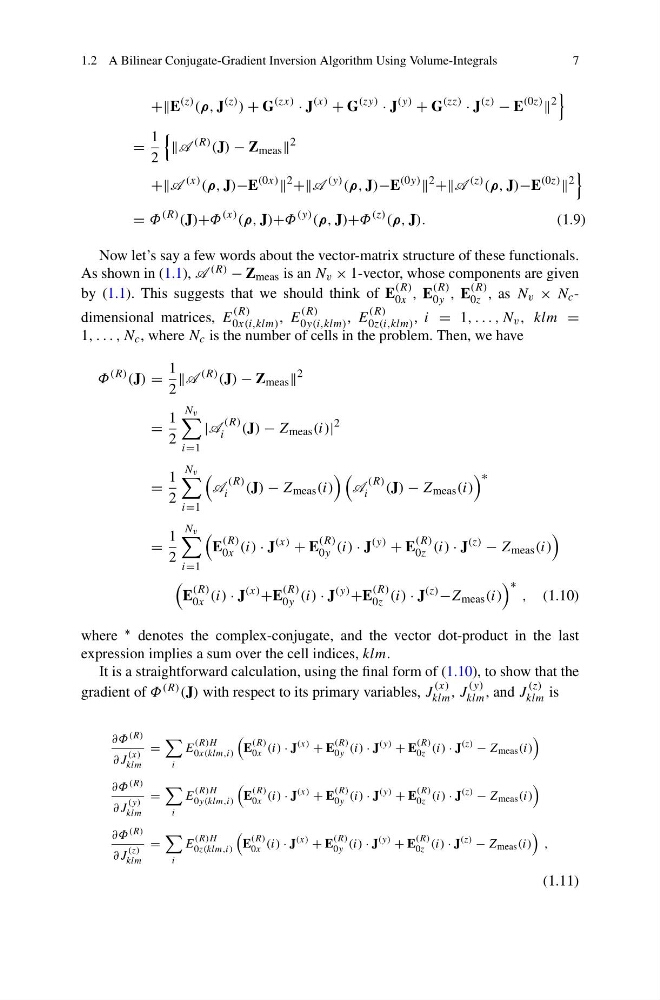
Now let’s say a few words about the vector-matrix structure of these functionals.
As shown in (1.1), A (R) − Z meas is an N v × 1-vector, whose components are given
by (1.1). This suggests that we should think of E
(R)
0x , E
(R)
0y , E
(R)
0z , as N v × N c -
dimensional matrices, E
(R)
0x(i,klm) , E
(R)
0y(i,klm) , E
(R)
0z(i,klm) , i = 1, . . . , N v , klm =
1, . . . , N c , where N c is the number of cells in the problem. Then, we have
Φ
(R) (J) =
1
2
A
(R) (J) − Z meas
2
=
1
2
N v
i=1
|A
(R)
i
(J) − Z meas (i)|
2
=
1
2
N v
i=1
A
(R)
i
(J) − Z meas (i)
A
(R)
i
(J) − Z meas (i)
∗
=
1
2
N v
i=1
E
(R)
0x (i) · J
(x)
+ E
(R)
0y (i) · J
(y)
+ E
(R)
0z (i) · J
(z)
− Z meas (i)
E
(R)
0x (i) · J
(x)
+E
(R)
0y (i) · J
(y)
+E
(R)
0z (i) · J
(z)
−Z meas (i)
∗
, (1.10)
where ∗ denotes the complex-conjugate, and the vector dot-product in the last
expression implies a sum over the cell indices, klm.
It is a straightforward calculation, using the final form of (1.10), to show that the
gradient of Φ (R) (J) with respect to its primary variables, J
(x)
klm , J
(y)
klm , and J
(z)
klm is
∂Φ (R)
∂J
(x)
klm
=
i
E
(R)H
0x(klm,i)
E
(R)
0x (i) · J
(x) + E
(R)
0y (i) · J
(y) + E
(R)
0z (i) · J
(z) − Z meas (i)
∂Φ (R)
∂J
(y)
klm
=
i
E
(R)H
0y(klm,i)
E
(R)
0x (i) · J
(x) + E
(R)
0y (i) · J
(y) + E
(R)
0z (i) · J
(z) − Z meas (i)
∂Φ (R)
∂J
(z)
klm
=
i
E
(R)H
0z(klm,i)
E
(R)
0x (i) · J
(x) + E
(R)
0y (i) · J
(y) + E
(R)
0z (i) · J
(z) − Z meas (i)
,
(1.11)
7
++E
(z) (ρ, J
(z) ) + G
(zx)
· J
(x)
+ G
(zy)
· J
(y)
+ G
(zz)
· J
(z)
− E
(0z)
2
=
1
2
A
(R) (J) − Z meas
2
++A
(x) (ρ, J)−E
(0x)
2
++A
(y) (ρ, J)−E
(0y)
2
++A
(z) (ρ, J)−E
(0z)
2
= Φ
(R) (J)+Φ
(x) (ρ, J)+Φ
(y) (ρ, J)+Φ
(z) (ρ, J).
(1.9)
Now let’s say a few words about the vector-matrix structure of these functionals.
As shown in (1.1), A (R) − Z meas is an N v × 1-vector, whose components are given
by (1.1). This suggests that we should think of E
(R)
0x , E
(R)
0y , E
(R)
0z , as N v × N c -
dimensional matrices, E
(R)
0x(i,klm) , E
(R)
0y(i,klm) , E
(R)
0z(i,klm) , i = 1, . . . , N v , klm =
1, . . . , N c , where N c is the number of cells in the problem. Then, we have
Φ
(R) (J) =
1
2
A
(R) (J) − Z meas
2
=
1
2
N v
i=1
|A
(R)
i
(J) − Z meas (i)|
2
=
1
2
N v
i=1
A
(R)
i
(J) − Z meas (i)
A
(R)
i
(J) − Z meas (i)
∗
=
1
2
N v
i=1
E
(R)
0x (i) · J
(x)
+ E
(R)
0y (i) · J
(y)
+ E
(R)
0z (i) · J
(z)
− Z meas (i)
E
(R)
0x (i) · J
(x)
+E
(R)
0y (i) · J
(y)
+E
(R)
0z (i) · J
(z)
−Z meas (i)
∗
, (1.10)
where ∗ denotes the complex-conjugate, and the vector dot-product in the last
expression implies a sum over the cell indices, klm.
It is a straightforward calculation, using the final form of (1.10), to show that the
gradient of Φ (R) (J) with respect to its primary variables, J
(x)
klm , J
(y)
klm , and J
(z)
klm is
∂Φ (R)
∂J
(x)
klm
=
i
E
(R)H
0x(klm,i)
E
(R)
0x (i) · J
(x) + E
(R)
0y (i) · J
(y) + E
(R)
0z (i) · J
(z) − Z meas (i)
∂Φ (R)
∂J
(y)
klm
=
i
E
(R)H
0y(klm,i)
E
(R)
0x (i) · J
(x) + E
(R)
0y (i) · J
(y) + E
(R)
0z (i) · J
(z) − Z meas (i)
∂Φ (R)
∂J
(z)
klm
=
i
E
(R)H
0z(klm,i)
E
(R)
0x (i) · J
(x) + E
(R)
0y (i) · J
(y) + E
(R)
0z (i) · J
(z) − Z meas (i)
,
(1.11)