

6
1 A Bilinear Conjugate-Gradient Inversion Algorithm
E
(y)
klm =
L
P
(y)
lL ρ kLm
E
(z)
klm =
M
P
(z)
mM ρ klM ,
(1.7)
where the matrix elements follow from (1.5) and (1.6)
P
(x)
kK (J (x) ) =
δxδyδz
6
J
(x)
k−1lm + 2J
(x)
klm if K = k
2J
(x)
klm + J
(x)
k+1lm if K = k + 1
P
(y)
lL (J (y) ) =
δxδyδz
6
J
(y)
kl−1m + 2J
(y)
klm if L = l
2J
(y)
klm + J
(y)
kl+1m if L = l + 1
P
(z)
mM (J (z) ) =
δxδyδz
6
J
(z)
klm−1 + 2J
(z)
klm if M = m
2J
(z)
klm + J
(z)
klm+1 if M = m + 1
(1.8)
One approach to solving the system, (1.1) and (1.4), has been to use a linear
(‘Born’) approximation, which means that the electric field within the flawed region
is assumed to be the same as the electric field if the flaw were not present, namely
the incident electric field. Thus, one would write J = σ E ≈ σ E 0 , and then take
moments of this equation. Substituting the resulting expressions for J
(x,y,z)
klm
into
(1.1) will produce a linear system for the unknown conductivities, σ klm , that can be
solved in a number of ways. See [105] for an example of this approach, in which
the linear system is solved using the algebraic reconstruction technique (ART), and
[24, 50, 51], as well as [111, pp. 282–285], for details on ART.
This approach, therefore, has the physical significance of ignoring the secondary
sources produced by multiple scattering within the flaw. From a mathematical
viewpoint, the second term of (1.4) (with the G matrices) is ignored. While
linearization is occasionally accurate, it is not as general as the main subject of this
chapter, bilinear conjugate-gradients. See [147] for a further discussion of the Born
approximation, and [14] for an application of the Born approximation to solve a
scattering problem of a three-dimensional flaw embedded in anisotropic composite
materials.
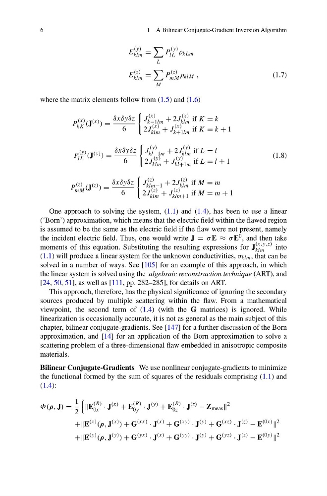
Bilinear Conjugate-Gradients We use nonlinear conjugate-gradients to minimize
the functional formed by the sum of squares of the residuals comprising (1.1) and
(1.4):
Φ(ρ, J) =
1
2
E
(R)
0x · J
(x)
+ E
(R)
0y · J
(y)
+ E
(R)
0z · J
(z)
− Z meas
2
++E
(x) (ρ, J
(x) ) + G
(xx)
· J
(x)
+ G
(xy)
· J
(y)
+ G
(xz)
· J
(z)
− E
(0x)
2
++E
(y) (ρ, J
(y) ) + G
(yx)
· J
(x)
+ G
(yy)
· J
(y)
+ G
(yz)
· J
(z)
− E
(0y)
2
1 A Bilinear Conjugate-Gradient Inversion Algorithm
E
(y)
klm =
L
P
(y)
lL ρ kLm
E
(z)
klm =
M
P
(z)
mM ρ klM ,
(1.7)
where the matrix elements follow from (1.5) and (1.6)
P
(x)
kK (J (x) ) =
δxδyδz
6
J
(x)
k−1lm + 2J
(x)
klm if K = k
2J
(x)
klm + J
(x)
k+1lm if K = k + 1
P
(y)
lL (J (y) ) =
δxδyδz
6
J
(y)
kl−1m + 2J
(y)
klm if L = l
2J
(y)
klm + J
(y)
kl+1m if L = l + 1
P
(z)
mM (J (z) ) =
δxδyδz
6
J
(z)
klm−1 + 2J
(z)
klm if M = m
2J
(z)
klm + J
(z)
klm+1 if M = m + 1
(1.8)
One approach to solving the system, (1.1) and (1.4), has been to use a linear
(‘Born’) approximation, which means that the electric field within the flawed region
is assumed to be the same as the electric field if the flaw were not present, namely
the incident electric field. Thus, one would write J = σ E ≈ σ E 0 , and then take
moments of this equation. Substituting the resulting expressions for J
(x,y,z)
klm
into
(1.1) will produce a linear system for the unknown conductivities, σ klm , that can be
solved in a number of ways. See [105] for an example of this approach, in which
the linear system is solved using the algebraic reconstruction technique (ART), and
[24, 50, 51], as well as [111, pp. 282–285], for details on ART.
This approach, therefore, has the physical significance of ignoring the secondary
sources produced by multiple scattering within the flaw. From a mathematical
viewpoint, the second term of (1.4) (with the G matrices) is ignored. While
linearization is occasionally accurate, it is not as general as the main subject of this
chapter, bilinear conjugate-gradients. See [147] for a further discussion of the Born
approximation, and [14] for an application of the Born approximation to solve a
scattering problem of a three-dimensional flaw embedded in anisotropic composite
materials.
Bilinear Conjugate-Gradients We use nonlinear conjugate-gradients to minimize
the functional formed by the sum of squares of the residuals comprising (1.1) and
(1.4):
Φ(ρ, J) =
1
2
E
(R)
0x · J
(x)
+ E
(R)
0y · J
(y)
+ E
(R)
0z · J
(z)
− Z meas
2
++E
(x) (ρ, J
(x) ) + G
(xx)
· J
(x)
+ G
(xy)
· J
(y)
+ G
(xz)
· J
(z)
− E
(0x)
2
++E
(y) (ρ, J
(y) ) + G
(yx)
· J
(x)
+ G
(yy)
· J
(y)
+ G
(yz)
· J
(z)
− E
(0y)
2