

1.2 A Bilinear Conjugate-Gradient Inversion Algorithm Using Volume-Integrals
5
⎡
⎣
E (0x)
E (0y)
E (0z)
⎤
⎦ =
⎡
⎣
E (x) (ρ, J (x) )
E (y) (ρ, J (y) )
E (z) (ρ, J (z) )
⎤
⎦ +
⎡
⎣
G (xx) G (xy) G (xz)
G (yx) G (yy) G (yz)
G (zx) G (zy) G (zz)
⎤
⎦
⎡
⎣
J (x)
J (y)
J (z)
⎤
⎦ .
(1.4)
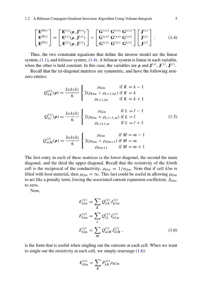
Thus, the two constraint equations that define the inverse model are the linear
system, (1.1), and bilinear system, (1.4). A bilinear system is linear in each variable,
when the other is held constant. In this case, the variables are ρ and J (x) , J (y) , J (z) .
Recall that the tri-diagonal matrices are symmetric, and have the following nonzero entries:
Q
(x)
kK (ρ) =
δxδyδz
6
⎧
⎨
⎩
ρ klm
if K = k − 1
2(ρ klm + ρ k+1,lm ) if K = k
ρ k+1,lm
if K = k + 1
Q
(y)
lL (ρ) =
δxδyδz
6
⎧
⎨
⎩
ρ klm
if L = l − 1
2(ρ klm + ρ k,l+1,m ) if L = l
ρ k,l+1,m
if L = l + 1
Q
(z)
mM (ρ) =
δxδyδz
6
⎧
⎨
⎩
ρ klm
if M = m − 1
2(ρ klm + ρ klm+1 ) if M = m
ρ klm+1
if M = m + 1
(1.5)
The first entry in each of these matrices is the lower diagonal, the second the main
diagonal, and the third the upper diagonal. Recall that the resistivity of the klmth
cell is the reciprocal of the conductivity, ρ klm = 1/σ klm . Note that if cell klm is
filled with host material, then ρ klm = ∞. This fact could be useful in allowing ρ klm
to act like a penalty term, forcing the associated current expansion coefficient, J klm ,
to zero.
Now,
E
(x)
klm =
K
Q
(x)
kK J
(x)
Klm
E
(y)
klm =
L
Q
(y)
lL J
(y)
kLm
E
(z)
klm =
M
Q
(z)
mM J
(z)
klM ,
(1.6)
is the form that is useful when singling out the currents at each cell. When we want
to single out the resistivity at each cell, we simply rearrange (1.6):
E
(x)
klm =
K
P
(x)
kK ρ Klm
5
⎡
⎣
E (0x)
E (0y)
E (0z)
⎤
⎦ =
⎡
⎣
E (x) (ρ, J (x) )
E (y) (ρ, J (y) )
E (z) (ρ, J (z) )
⎤
⎦ +
⎡
⎣
G (xx) G (xy) G (xz)
G (yx) G (yy) G (yz)
G (zx) G (zy) G (zz)
⎤
⎦
⎡
⎣
J (x)
J (y)
J (z)
⎤
⎦ .
(1.4)
Thus, the two constraint equations that define the inverse model are the linear
system, (1.1), and bilinear system, (1.4). A bilinear system is linear in each variable,
when the other is held constant. In this case, the variables are ρ and J (x) , J (y) , J (z) .
Recall that the tri-diagonal matrices are symmetric, and have the following nonzero entries:
Q
(x)
kK (ρ) =
δxδyδz
6
⎧
⎨
⎩
ρ klm
if K = k − 1
2(ρ klm + ρ k+1,lm ) if K = k
ρ k+1,lm
if K = k + 1
Q
(y)
lL (ρ) =
δxδyδz
6
⎧
⎨
⎩
ρ klm
if L = l − 1
2(ρ klm + ρ k,l+1,m ) if L = l
ρ k,l+1,m
if L = l + 1
Q
(z)
mM (ρ) =
δxδyδz
6
⎧
⎨
⎩
ρ klm
if M = m − 1
2(ρ klm + ρ klm+1 ) if M = m
ρ klm+1
if M = m + 1
(1.5)
The first entry in each of these matrices is the lower diagonal, the second the main
diagonal, and the third the upper diagonal. Recall that the resistivity of the klmth
cell is the reciprocal of the conductivity, ρ klm = 1/σ klm . Note that if cell klm is
filled with host material, then ρ klm = ∞. This fact could be useful in allowing ρ klm
to act like a penalty term, forcing the associated current expansion coefficient, J klm ,
to zero.
Now,
E
(x)
klm =
K
Q
(x)
kK J
(x)
Klm
E
(y)
klm =
L
Q
(y)
lL J
(y)
kLm
E
(z)
klm =
M
Q
(z)
mM J
(z)
klM ,
(1.6)
is the form that is useful when singling out the currents at each cell. When we want
to single out the resistivity at each cell, we simply rearrange (1.6):
E
(x)
klm =
K
P
(x)
kK ρ Klm