

4
1 A Bilinear Conjugate-Gradient Inversion Algorithm
and an array of N v receive coils occupying the positions of the original scanned
receive coil. Furthermore, we could actually scan fewer than N v positions, and
then interpolate to complete the N v data points. (See [107] and [14] for further
discussions of multiview and multifrequency reconstruction methods.)
In any case, the transmitter generates an anomalous scattering current,
J (x) , J (y) , J (z) , which is computed by VIC-3D ® and the receive coil(s) produces
an incident field, E
(R)
0x (i), E
(R)
0y (i), E
(R)
0z (i). These combine to produce the changein-transfer impedance due to the anomaly,
Z
(i) (J) = E
(R)
0x (i) · J
(x)
+ E
(R)
0y (i) · J
(y)
+ E
(R)
0z (i) · J
(z) ,
(1.1)
that is also computed directly by VIC-3D ® . 1 Note that, unlike our NLSE algorithm,
we do not consider J (x) , J (y) , J (z) to be secondary variables that are dependent upon
the primary unknown, σ . Rather, the current-vectors along with the cell resistivities,
ρ, are the primary unknowns.
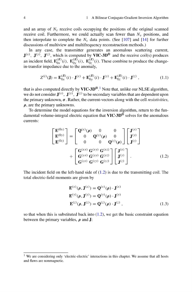
To determine the model equations for the inversion algorithm, return to the fundamental volume-integral electric equation that VIC-3D ® solves for the anomalous
currents:
⎡
⎣
E (0x)
E (0y)
E (0z)
⎤
⎦ =
⎡
⎣
Q (x) (ρ)
0
0
0
Q (y) (ρ)
0
0
0
Q (z) (ρ)
⎤
⎦
⎡
⎣
J (x)
J (y)
J (z)
⎤
⎦
+
⎡
⎣
G (xx) G (xy) G (xz)
G (yx) G (yy) G (yz)
G (zx) G (zy) G (zz)
⎤
⎦
⎡
⎣
J (x)
J (y)
J (z)
⎤
⎦ .
(1.2)
The incident field on the left-hand side of (1.2) is due to the transmitting coil. The
total electric-field moments are given by
E
(x) (ρ, J
(x) ) = Q
(x) (ρ) · J
(x)
E
(y) (ρ, J
(y) ) = Q
(y) (ρ) · J
(y)
E
(z) (ρ, J
(z) ) = Q
(z) (ρ) · J
(z) ,
(1.3)
so that when this is substituted back into (1.2), we get the basic constraint equation
between the primary variables, ρ and J:
1 We are considering only ‘electric-electric’ interactions in this chapter. We assume that all hosts
and flaws are nonmagnetic.
1 A Bilinear Conjugate-Gradient Inversion Algorithm
and an array of N v receive coils occupying the positions of the original scanned
receive coil. Furthermore, we could actually scan fewer than N v positions, and
then interpolate to complete the N v data points. (See [107] and [14] for further
discussions of multiview and multifrequency reconstruction methods.)
In any case, the transmitter generates an anomalous scattering current,
J (x) , J (y) , J (z) , which is computed by VIC-3D ® and the receive coil(s) produces
an incident field, E
(R)
0x (i), E
(R)
0y (i), E
(R)
0z (i). These combine to produce the changein-transfer impedance due to the anomaly,
Z
(i) (J) = E
(R)
0x (i) · J
(x)
+ E
(R)
0y (i) · J
(y)
+ E
(R)
0z (i) · J
(z) ,
(1.1)
that is also computed directly by VIC-3D ® . 1 Note that, unlike our NLSE algorithm,
we do not consider J (x) , J (y) , J (z) to be secondary variables that are dependent upon
the primary unknown, σ . Rather, the current-vectors along with the cell resistivities,
ρ, are the primary unknowns.
To determine the model equations for the inversion algorithm, return to the fundamental volume-integral electric equation that VIC-3D ® solves for the anomalous
currents:
⎡
⎣
E (0x)
E (0y)
E (0z)
⎤
⎦ =
⎡
⎣
Q (x) (ρ)
0
0
0
Q (y) (ρ)
0
0
0
Q (z) (ρ)
⎤
⎦
⎡
⎣
J (x)
J (y)
J (z)
⎤
⎦
+
⎡
⎣
G (xx) G (xy) G (xz)
G (yx) G (yy) G (yz)
G (zx) G (zy) G (zz)
⎤
⎦
⎡
⎣
J (x)
J (y)
J (z)
⎤
⎦ .
(1.2)
The incident field on the left-hand side of (1.2) is due to the transmitting coil. The
total electric-field moments are given by
E
(x) (ρ, J
(x) ) = Q
(x) (ρ) · J
(x)
E
(y) (ρ, J
(y) ) = Q
(y) (ρ) · J
(y)
E
(z) (ρ, J
(z) ) = Q
(z) (ρ) · J
(z) ,
(1.3)
so that when this is substituted back into (1.2), we get the basic constraint equation
between the primary variables, ρ and J:
1 We are considering only ‘electric-electric’ interactions in this chapter. We assume that all hosts
and flaws are nonmagnetic.