

162
7 Integration of Functionals, PCM and Stochastic IntegralEquations
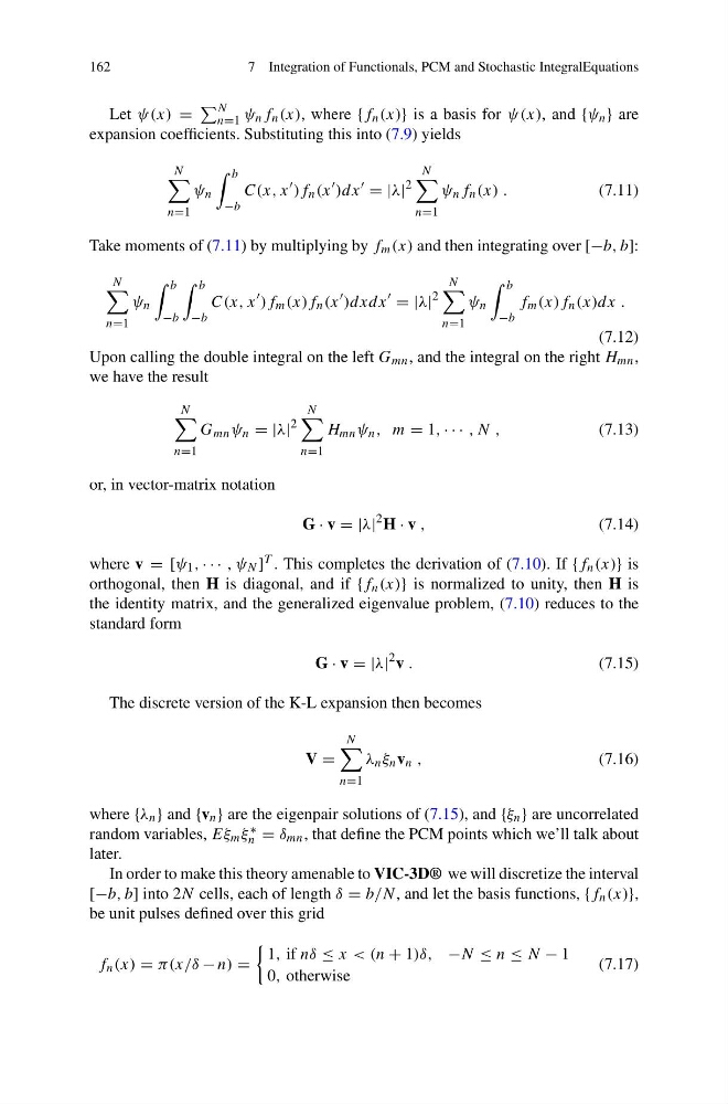
Let ψ(x) =
N
n=1 ψ n f n (x), where {f n (x)} is a basis for ψ(x), and {ψ n } are
expansion coefficients. Substituting this into (7.9) yields
N
n=1
ψ n
b
−b
C(x, x
)f n (x
)dx
= |λ|
2
N
n=1
ψ n f n (x) .
(7.11)
Take moments of (7.11) by multiplying by f m (x) and then integrating over [−b, b]:
N
n=1
ψ n
b
−b
b
−b
C(x, x
)f m (x)f n (x
)dxdx
= |λ|
2
N
n=1
ψ n
b
−b
f m (x)f n (x)dx .
(7.12)
Upon calling the double integral on the left G mn , and the integral on the right H mn ,
we have the result
N
n=1
G mn ψ n = |λ|
2
N
n=1
H mn ψ n , m = 1, · · · , N ,
(7.13)
or, in vector-matrix notation
G · v = |λ|
2 H · v ,
(7.14)
where v = [ψ 1 , · · · , ψ N ] T . This completes the derivation of (7.10). If {f n (x)} is
orthogonal, then H is diagonal, and if {f n (x)} is normalized to unity, then H is
the identity matrix, and the generalized eigenvalue problem, (7.10) reduces to the
standard form
G · v = |λ|
2 v .
(7.15)
The discrete version of the K-L expansion then becomes
V =
N
n=1
λ n ξ n v n ,
(7.16)
where {λ n } and {v n } are the eigenpair solutions of (7.15), and {ξ n } are uncorrelated
random variables, Eξ m ξ ∗
n = δ mn , that define the PCM points which we’ll talk about
later.
In order to make this theory amenable to VIC-3D® we will discretize the interval
[−b, b] into 2N cells, each of length δ = b/N, and let the basis functions, {f n (x)},
be unit pulses defined over this grid
f n (x) = π(x/δ − n) =
1, if nδ ≤ x < (n + 1)δ, −N ≤ n ≤ N − 1
0, otherwise
(7.17)
7 Integration of Functionals, PCM and Stochastic IntegralEquations
Let ψ(x) =
N
n=1 ψ n f n (x), where {f n (x)} is a basis for ψ(x), and {ψ n } are
expansion coefficients. Substituting this into (7.9) yields
N
n=1
ψ n
b
−b
C(x, x
)f n (x
)dx
= |λ|
2
N
n=1
ψ n f n (x) .
(7.11)
Take moments of (7.11) by multiplying by f m (x) and then integrating over [−b, b]:
N
n=1
ψ n
b
−b
b
−b
C(x, x
)f m (x)f n (x
)dxdx
= |λ|
2
N
n=1
ψ n
b
−b
f m (x)f n (x)dx .
(7.12)
Upon calling the double integral on the left G mn , and the integral on the right H mn ,
we have the result
N
n=1
G mn ψ n = |λ|
2
N
n=1
H mn ψ n , m = 1, · · · , N ,
(7.13)
or, in vector-matrix notation
G · v = |λ|
2 H · v ,
(7.14)
where v = [ψ 1 , · · · , ψ N ] T . This completes the derivation of (7.10). If {f n (x)} is
orthogonal, then H is diagonal, and if {f n (x)} is normalized to unity, then H is
the identity matrix, and the generalized eigenvalue problem, (7.10) reduces to the
standard form
G · v = |λ|
2 v .
(7.15)
The discrete version of the K-L expansion then becomes
V =
N
n=1
λ n ξ n v n ,
(7.16)
where {λ n } and {v n } are the eigenpair solutions of (7.15), and {ξ n } are uncorrelated
random variables, Eξ m ξ ∗
n = δ mn , that define the PCM points which we’ll talk about
later.
In order to make this theory amenable to VIC-3D® we will discretize the interval
[−b, b] into 2N cells, each of length δ = b/N, and let the basis functions, {f n (x)},
be unit pulses defined over this grid
f n (x) = π(x/δ − n) =
1, if nδ ≤ x < (n + 1)δ, −N ≤ n ≤ N − 1
0, otherwise
(7.17)