

7.4 A One-Dimensional Random Surface
161
Almen 2A
Almen 8A
Distance [mm]
Distance [mm]
1
0.8
0.6
0.4
0.2
0
1
0.8
0.6
0.4
0.2
0
-0.5
-0.25
0
0.25
0.5
-0.5
-0.25
0
0.25
0.5
Correlation Function
Correlation Function
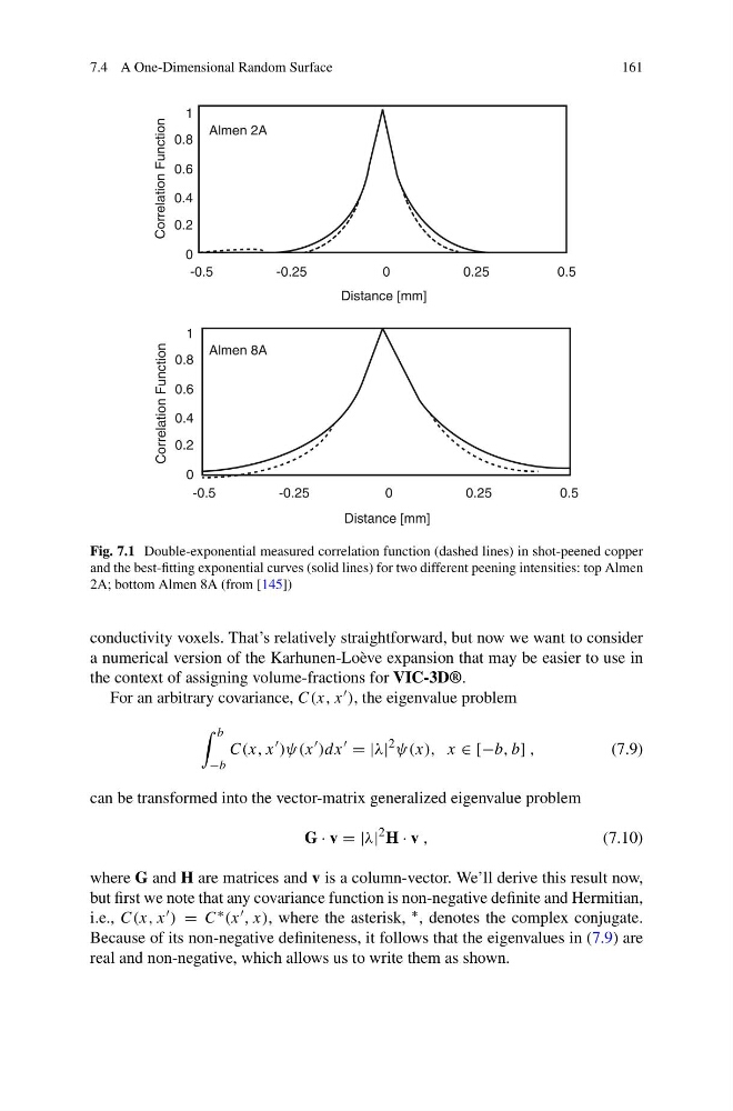
Fig. 7.1 Double-exponential measured correlation function (dashed lines) in shot-peened copper
and the best-fitting exponential curves (solid lines) for two different peening intensities: top Almen
2A; bottom Almen 8A (from [145])
conductivity voxels. That’s relatively straightforward, but now we want to consider
a numerical version of the Karhunen-Loève expansion that may be easier to use in
the context of assigning volume-fractions for VIC-3D®.
For an arbitrary covariance, C(x, x ), the eigenvalue problem
b
−b
C(x, x
)ψ(x
)dx
= |λ|
2 ψ(x), x ∈ [−b, b] ,
(7.9)
can be transformed into the vector-matrix generalized eigenvalue problem
G · v = |λ|
2 H · v ,
(7.10)
where G and H are matrices and v is a column-vector. We’ll derive this result now,
but first we note that any covariance function is non-negative definite and Hermitian,
i.e., C(x, x ) = C ∗ (x , x), where the asterisk, ∗ , denotes the complex conjugate.
Because of its non-negative definiteness, it follows that the eigenvalues in (7.9) are
real and non-negative, which allows us to write them as shown.
161
Almen 2A
Almen 8A
Distance [mm]
Distance [mm]
1
0.8
0.6
0.4
0.2
0
1
0.8
0.6
0.4
0.2
0
-0.5
-0.25
0
0.25
0.5
-0.5
-0.25
0
0.25
0.5
Correlation Function
Correlation Function
Fig. 7.1 Double-exponential measured correlation function (dashed lines) in shot-peened copper
and the best-fitting exponential curves (solid lines) for two different peening intensities: top Almen
2A; bottom Almen 8A (from [145])
conductivity voxels. That’s relatively straightforward, but now we want to consider
a numerical version of the Karhunen-Loève expansion that may be easier to use in
the context of assigning volume-fractions for VIC-3D®.
For an arbitrary covariance, C(x, x ), the eigenvalue problem
b
−b
C(x, x
)ψ(x
)dx
= |λ|
2 ψ(x), x ∈ [−b, b] ,
(7.9)
can be transformed into the vector-matrix generalized eigenvalue problem
G · v = |λ|
2 H · v ,
(7.10)
where G and H are matrices and v is a column-vector. We’ll derive this result now,
but first we note that any covariance function is non-negative definite and Hermitian,
i.e., C(x, x ) = C ∗ (x , x), where the asterisk, ∗ , denotes the complex conjugate.
Because of its non-negative definiteness, it follows that the eigenvalues in (7.9) are
real and non-negative, which allows us to write them as shown.