

154
6 Stochastic Inverse Problems: Models and Metrics
Table 6.3 Inverted results
for the width of a crack
Trial r(x) max
r(x ∗ )
W/sensit
1
0.7979(−1) 0.2495(−1) 0.0793/0.0296
2
0.7990(−1) 0.2495(−1) 0.0793/0.0296
3
0.8024(−1) 0.2495(−1) 0.0793/0.0296
4
0.7941(−1) 0.2495(−1) 0.0793/0.0296
5
0.7999(−1) 0.2495(−1) 0.0793/0.0296
Following the procedure described above with respect to the Chebyshev inequality, we calculate a value of = 137, which yields σ cond = 0.272 × 10 6 , and
σ μ = 1.76. Hence, we can say that the most likely value of the conductivity is
1.372 × 10 6 , with a 95% confidence interval of [1.1 × 10 6 , 1.644 × 10 6 ]. For the
permeability we get even tighter results; the most likely value is 68.18, with a 95%
confidence interval of [66.42, 69.94].
The fact that the permeability is well defined at these low frequencies has been
validated by use of the Cramer-Rao Lower Bound (CRLB), [111, pp. 407–410],
where it is also shown that the optimum frequency for estimating conductivity is
6.0 kHz.
Estimation of Width of a Long, Thin Crack We are given data at 200 kHz for a
crack in a bolt-hole. The data were obtained by a splitD probe with ferrite cores, and
the crack was 100 mils long and 18 mils deep. The objective was to determine the
width of the crack. The problem is described in greater detail in [111, Section 6.6].
The interpolation table for the width has nodes at 0, 0.125 mils, and 0.25 mils.
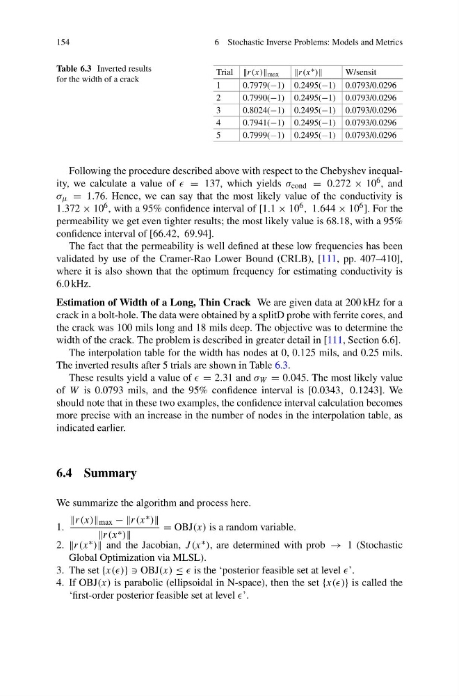
The inverted results after 5 trials are shown in Table 6.3.
These results yield a value of = 2.31 and σ W = 0.045. The most likely value
of W is 0.0793 mils, and the 95% confidence interval is [0.0343, 0.1243]. We
should note that in these two examples, the confidence interval calculation becomes
more precise with an increase in the number of nodes in the interpolation table, as
indicated earlier.
6.4 Summary
We summarize the algorithm and process here.
1.
r(x) max − −r(x ∗ )
r(x ∗ )
= OBJ(x) is a random variable.
2. r(x ∗ ) and the Jacobian, J (x ∗ ), are determined with prob → 1 (Stochastic
Global Optimization via MLSL).
3. The set {x(()} } OBJ(x) ≤ is the ‘posterior feasible set at level ’.
4. If OBJ(x) is parabolic (ellipsoidal in N-space), then the set {x(()} is called the
‘first-order posterior feasible set at level ’.
6 Stochastic Inverse Problems: Models and Metrics
Table 6.3 Inverted results
for the width of a crack
Trial r(x) max
r(x ∗ )
W/sensit
1
0.7979(−1) 0.2495(−1) 0.0793/0.0296
2
0.7990(−1) 0.2495(−1) 0.0793/0.0296
3
0.8024(−1) 0.2495(−1) 0.0793/0.0296
4
0.7941(−1) 0.2495(−1) 0.0793/0.0296
5
0.7999(−1) 0.2495(−1) 0.0793/0.0296
Following the procedure described above with respect to the Chebyshev inequality, we calculate a value of = 137, which yields σ cond = 0.272 × 10 6 , and
σ μ = 1.76. Hence, we can say that the most likely value of the conductivity is
1.372 × 10 6 , with a 95% confidence interval of [1.1 × 10 6 , 1.644 × 10 6 ]. For the
permeability we get even tighter results; the most likely value is 68.18, with a 95%
confidence interval of [66.42, 69.94].
The fact that the permeability is well defined at these low frequencies has been
validated by use of the Cramer-Rao Lower Bound (CRLB), [111, pp. 407–410],
where it is also shown that the optimum frequency for estimating conductivity is
6.0 kHz.
Estimation of Width of a Long, Thin Crack We are given data at 200 kHz for a
crack in a bolt-hole. The data were obtained by a splitD probe with ferrite cores, and
the crack was 100 mils long and 18 mils deep. The objective was to determine the
width of the crack. The problem is described in greater detail in [111, Section 6.6].
The interpolation table for the width has nodes at 0, 0.125 mils, and 0.25 mils.
The inverted results after 5 trials are shown in Table 6.3.
These results yield a value of = 2.31 and σ W = 0.045. The most likely value
of W is 0.0793 mils, and the 95% confidence interval is [0.0343, 0.1243]. We
should note that in these two examples, the confidence interval calculation becomes
more precise with an increase in the number of nodes in the interpolation table, as
indicated earlier.
6.4 Summary
We summarize the algorithm and process here.
1.
r(x) max − −r(x ∗ )
r(x ∗ )
= OBJ(x) is a random variable.
2. r(x ∗ ) and the Jacobian, J (x ∗ ), are determined with prob → 1 (Stochastic
Global Optimization via MLSL).
3. The set {x(()} } OBJ(x) ≤ is the ‘posterior feasible set at level ’.
4. If OBJ(x) is parabolic (ellipsoidal in N-space), then the set {x(()} is called the
‘first-order posterior feasible set at level ’.