

6.3 Confidence Levels: Stochastic Global Optimization
153
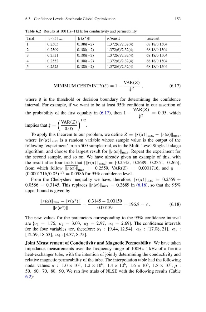
Table 6.2 Results at 100 Hz–1 kHz for conductivity and permeability
Trial
r(x) max
r(x ∗ )
σ /sensit
μ/sensit
1
0.2503
0.188(−2)
1.372(6)/2.32(4)
68.18/0.1504
2
0.2509
0.188(−2)
1.372(6)/2.32(4)
68.18/0.1504
3
0.2521
0.188(−2)
1.372(6)/2.32(4)
68.18/0.1504
4
0.2552
0.188(−2)
1.372(6)/2.32(4)
68.18/0.1504
5
0.2525
0.188(−2)
1.372(6)/2.32(4)
68.18/0.1504
MINIMUM CERTAINTY(ξ ) = 1 −
VAR(Z)
ξ 2
,
(6.17)
where ξ is the threshold or decision boundary for determining the confidence
interval. For example, if we want to be at least 95% confident in our assertion of
the probability of the first equality in (6.17), then 1 −
VAR(Z)
ξ 2
= 0.95, which
implies that ξ =
VAR(Z)
0.05
1/2
.
To apply this theorem to our problem, we define Z = =r(α) max − r(α) max ,
where r(α) max is a random variable whose sample value is the output of the
following ‘experiment’: run a 500-sample trial, as in the Multi-Level Single Linkage
algorithm, and choose the largest result for r(α) max . Repeat the experiment for
the second sample, and so on. We have already given an example of this, with
the result after four trials that {{r(α) max } = {0.2545, 0.2689, 0.2351, 0.265},
from which follow r(α) max = 0.2559, VAR(Z) = 0.0001716, and ξ =
(0.0001716/0.05)
1/2
= 0.0586 for 95% confidence level.
From the Chebyshev inequality we have, therefore, r(α) max = 0.2559 +
0.0586 = 0.3145. This replaces r(α) max = 0.2689 in (6.16), so that the 95%
upper bound is given by
r(α) max − −r(α ∗ )
r(α ∗ )
=
0.3145 − 0.00159
0.00159
= 196.8 = .
(6.18)
The new values for the parameters corresponding to the 95% confidence interval
are {σ 1 = 1.75, σ 2 = 3.03, σ 3 = 2.97, σ 4 = 2.69}. The confidence intervals
for the four variables are, therefore: α 1 : [9.44, 12.94], α 2 : [17.08, 21], α 3 :
[12.59, 18.53], α 4 : [3.37, 8.75].
Joint Measurement of Conductivity and Magnetic Permeability We have taken
impedance measurements over the frequency range of 100Hz–1 kHz of a ferritic
heat-exchanger tube, with the intention of jointly determining the conductivity and
relative magnetic permeability of the tube. The interpolation table had the following
nodal values: σ : 1.0 × 10 6 , 1.2 × 10 6 , 1.4 × 10 6 , 1.6 × 10 6 , 1.8 × 10 6 ; μ :
50, 60, 70, 80, 90. We ran five trials of NLSE with the following results (Table
6.2):
153
Table 6.2 Results at 100 Hz–1 kHz for conductivity and permeability
Trial
r(x) max
r(x ∗ )
σ /sensit
μ/sensit
1
0.2503
0.188(−2)
1.372(6)/2.32(4)
68.18/0.1504
2
0.2509
0.188(−2)
1.372(6)/2.32(4)
68.18/0.1504
3
0.2521
0.188(−2)
1.372(6)/2.32(4)
68.18/0.1504
4
0.2552
0.188(−2)
1.372(6)/2.32(4)
68.18/0.1504
5
0.2525
0.188(−2)
1.372(6)/2.32(4)
68.18/0.1504
MINIMUM CERTAINTY(ξ ) = 1 −
VAR(Z)
ξ 2
,
(6.17)
where ξ is the threshold or decision boundary for determining the confidence
interval. For example, if we want to be at least 95% confident in our assertion of
the probability of the first equality in (6.17), then 1 −
VAR(Z)
ξ 2
= 0.95, which
implies that ξ =
VAR(Z)
0.05
1/2
.
To apply this theorem to our problem, we define Z = =r(α) max − r(α) max ,
where r(α) max is a random variable whose sample value is the output of the
following ‘experiment’: run a 500-sample trial, as in the Multi-Level Single Linkage
algorithm, and choose the largest result for r(α) max . Repeat the experiment for
the second sample, and so on. We have already given an example of this, with
the result after four trials that {{r(α) max } = {0.2545, 0.2689, 0.2351, 0.265},
from which follow r(α) max = 0.2559, VAR(Z) = 0.0001716, and ξ =
(0.0001716/0.05)
1/2
= 0.0586 for 95% confidence level.
From the Chebyshev inequality we have, therefore, r(α) max = 0.2559 +
0.0586 = 0.3145. This replaces r(α) max = 0.2689 in (6.16), so that the 95%
upper bound is given by
r(α) max − −r(α ∗ )
r(α ∗ )
=
0.3145 − 0.00159
0.00159
= 196.8 = .
(6.18)
The new values for the parameters corresponding to the 95% confidence interval
are {σ 1 = 1.75, σ 2 = 3.03, σ 3 = 2.97, σ 4 = 2.69}. The confidence intervals
for the four variables are, therefore: α 1 : [9.44, 12.94], α 2 : [17.08, 21], α 3 :
[12.59, 18.53], α 4 : [3.37, 8.75].
Joint Measurement of Conductivity and Magnetic Permeability We have taken
impedance measurements over the frequency range of 100Hz–1 kHz of a ferritic
heat-exchanger tube, with the intention of jointly determining the conductivity and
relative magnetic permeability of the tube. The interpolation table had the following
nodal values: σ : 1.0 × 10 6 , 1.2 × 10 6 , 1.4 × 10 6 , 1.6 × 10 6 , 1.8 × 10 6 ; μ :
50, 60, 70, 80, 90. We ran five trials of NLSE with the following results (Table
6.2):