

152
6 Stochastic Inverse Problems: Models and Metrics
0
0.05
0.1
0.15
0.2
0.25
2
2.5
3
3.5
4
Nodes per Dimension
Stochastic Estimation Metrics vs. Number of Nodes
r
sensit1
sensit2
sensit3
sensit4
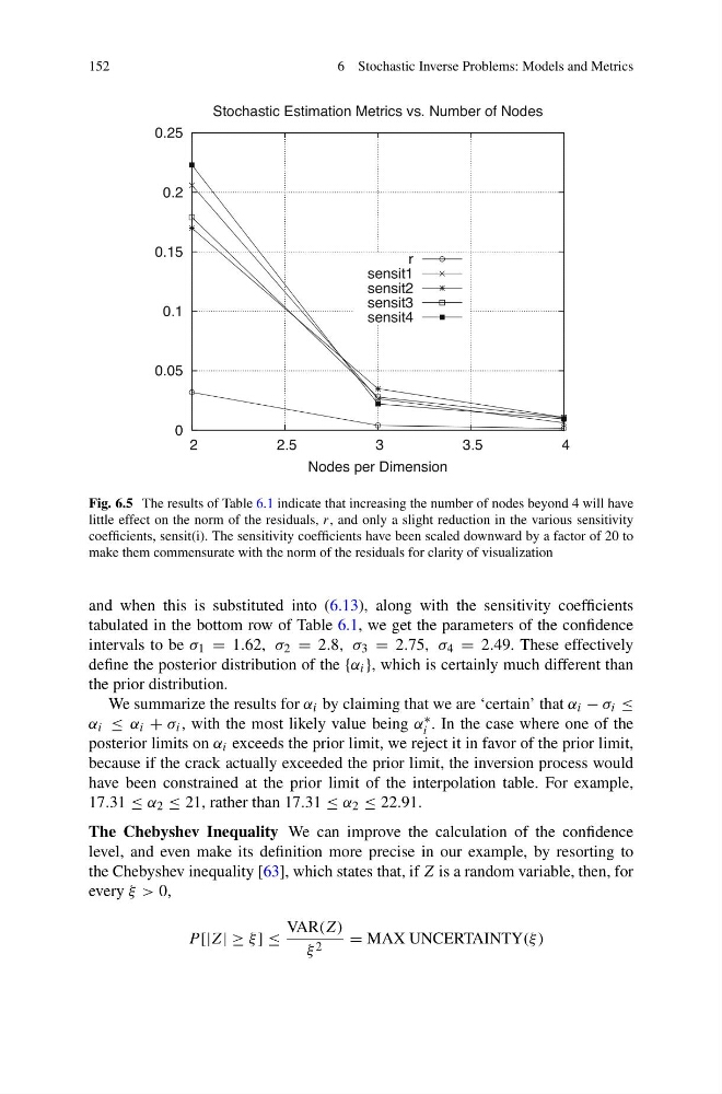
Fig. 6.5 The results of Table 6.1 indicate that increasing the number of nodes beyond 4 will have
little effect on the norm of the residuals, r, and only a slight reduction in the various sensitivity
coefficients, sensit(i). The sensitivity coefficients have been scaled downward by a factor of 20 to
make them commensurate with the norm of the residuals for clarity of visualization
and when this is substituted into (6.13), along with the sensitivity coefficients
tabulated in the bottom row of Table 6.1, we get the parameters of the confidence
intervals to be σ 1 = 1.62, σ 2 = 2.8, σ 3 = 2.75, σ 4 = 2.49. These effectively
define the posterior distribution of the {α i }, which is certainly much different than
the prior distribution.
We summarize the results for α i by claiming that we are ‘certain’ that α i − σ i ≤
α i ≤ α i + σ i , with the most likely value being α ∗
i . In the case where one of the
posterior limits on α i exceeds the prior limit, we reject it in favor of the prior limit,
because if the crack actually exceeded the prior limit, the inversion process would
have been constrained at the prior limit of the interpolation table. For example,
17.31 ≤ α 2 ≤ 21, rather than 17.31 ≤ α 2 ≤ 22.91.
The Chebyshev Inequality We can improve the calculation of the confidence
level, and even make its definition more precise in our example, by resorting to
the Chebyshev inequality [63], which states that, if Z is a random variable, then, for
every ξ > 0,
P [|Z| ≥ ξ ] ≤
VAR(Z)
ξ 2
= MAX UNCERTAINTY(ξ )
6 Stochastic Inverse Problems: Models and Metrics
0
0.05
0.1
0.15
0.2
0.25
2
2.5
3
3.5
4
Nodes per Dimension
Stochastic Estimation Metrics vs. Number of Nodes
r
sensit1
sensit2
sensit3
sensit4
Fig. 6.5 The results of Table 6.1 indicate that increasing the number of nodes beyond 4 will have
little effect on the norm of the residuals, r, and only a slight reduction in the various sensitivity
coefficients, sensit(i). The sensitivity coefficients have been scaled downward by a factor of 20 to
make them commensurate with the norm of the residuals for clarity of visualization
and when this is substituted into (6.13), along with the sensitivity coefficients
tabulated in the bottom row of Table 6.1, we get the parameters of the confidence
intervals to be σ 1 = 1.62, σ 2 = 2.8, σ 3 = 2.75, σ 4 = 2.49. These effectively
define the posterior distribution of the {α i }, which is certainly much different than
the prior distribution.
We summarize the results for α i by claiming that we are ‘certain’ that α i − σ i ≤
α i ≤ α i + σ i , with the most likely value being α ∗
i . In the case where one of the
posterior limits on α i exceeds the prior limit, we reject it in favor of the prior limit,
because if the crack actually exceeded the prior limit, the inversion process would
have been constrained at the prior limit of the interpolation table. For example,
17.31 ≤ α 2 ≤ 21, rather than 17.31 ≤ α 2 ≤ 22.91.
The Chebyshev Inequality We can improve the calculation of the confidence
level, and even make its definition more precise in our example, by resorting to
the Chebyshev inequality [63], which states that, if Z is a random variable, then, for
every ξ > 0,
P [|Z| ≥ ξ ] ≤
VAR(Z)
ξ 2
= MAX UNCERTAINTY(ξ )