

6.3 Confidence Levels: Stochastic Global Optimization
151
1
2
3
Y
Z
20 mil
−25
25
50
Width of anomaly = 0.1mil
mil
mil
−50
10 mil
mil
mil
4
15 mil
5 mil
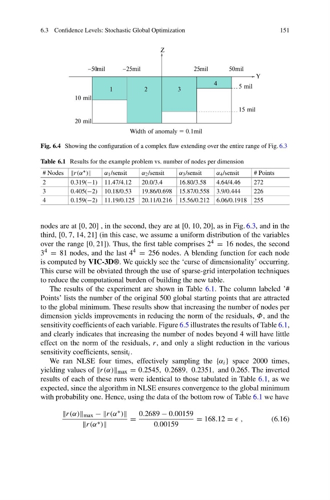
Fig. 6.4 Showing the configuration of a complex flaw extending over the entire range of Fig. 6.3
Table 6.1 Results for the example problem vs. number of nodes per dimension
# Nodes r(α ∗ )
α 1 /sensit
α 2 /sensit
α 3 /sensit
α 4 /sensit
# Points
2
0.319(−1) 11.47/4.12
20.0/3.4
16.80/3.58
4.64/4.46
272
3
0.405(−2) 10.18/0.53
19.86/0.698 15.87/0.558 3.9/0.444
226
4
0.159(−2) 11.19/0.125 20.11/0.216 15.56/0.212 6.06/0.1918 255
nodes are at [0, 20] , in the second, they are at [0, 10, 20], as in Fig. 6.3, and in the
third, [0, 7, 14, 21] (in this case, we assume a uniform distribution of the variables
over the range [0, 21]). Thus, the first table comprises 2 4 = 16 nodes, the second
3 4 = 81 nodes, and the last 4 4 = 256 nodes. A blending function for each node
is computed by VIC-3D®. We quickly see the ‘curse of dimensionality’ occurring.
This curse will be obviated through the use of sparse-grid interpolation techniques
to reduce the computational burden of building the new table.
The results of the experiment are shown in Table 6.1. The column labeled ’#
Points’ lists the number of the original 500 global starting points that are attracted
to the global minimum. These results show that increasing the number of nodes per
dimension yields improvements in reducing the norm of the residuals, Φ, and the
sensitivity coefficients of each variable. Figure 6.5 illustrates the results of Table 6.1,
and clearly indicates that increasing the number of nodes beyond 4 will have little
effect on the norm of the residuals, r, and only a slight reduction in the various
sensitivity coefficients, sensit i .
We ran NLSE four times, effectively sampling the {α i } space 2000 times,
yielding values of r(α) max = 0.2545, 0.2689, 0.2351, and 0.265. The inverted
results of each of these runs were identical to those tabulated in Table 6.1, as we
expected, since the algorithm in NLSE ensures convergence to the global minimum
with probability one. Hence, using the data of the bottom row of Table 6.1 we have
r(α) max − −r(α ∗ )
r(α ∗ )
=
0.2689 − 0.00159
0.00159
= 168.12 = ,
(6.16)
151
1
2
3
Y
Z
20 mil
−25
25
50
Width of anomaly = 0.1mil
mil
mil
−50
10 mil
mil
mil
4
15 mil
5 mil
Fig. 6.4 Showing the configuration of a complex flaw extending over the entire range of Fig. 6.3
Table 6.1 Results for the example problem vs. number of nodes per dimension
# Nodes r(α ∗ )
α 1 /sensit
α 2 /sensit
α 3 /sensit
α 4 /sensit
# Points
2
0.319(−1) 11.47/4.12
20.0/3.4
16.80/3.58
4.64/4.46
272
3
0.405(−2) 10.18/0.53
19.86/0.698 15.87/0.558 3.9/0.444
226
4
0.159(−2) 11.19/0.125 20.11/0.216 15.56/0.212 6.06/0.1918 255
nodes are at [0, 20] , in the second, they are at [0, 10, 20], as in Fig. 6.3, and in the
third, [0, 7, 14, 21] (in this case, we assume a uniform distribution of the variables
over the range [0, 21]). Thus, the first table comprises 2 4 = 16 nodes, the second
3 4 = 81 nodes, and the last 4 4 = 256 nodes. A blending function for each node
is computed by VIC-3D®. We quickly see the ‘curse of dimensionality’ occurring.
This curse will be obviated through the use of sparse-grid interpolation techniques
to reduce the computational burden of building the new table.
The results of the experiment are shown in Table 6.1. The column labeled ’#
Points’ lists the number of the original 500 global starting points that are attracted
to the global minimum. These results show that increasing the number of nodes per
dimension yields improvements in reducing the norm of the residuals, Φ, and the
sensitivity coefficients of each variable. Figure 6.5 illustrates the results of Table 6.1,
and clearly indicates that increasing the number of nodes beyond 4 will have little
effect on the norm of the residuals, r, and only a slight reduction in the various
sensitivity coefficients, sensit i .
We ran NLSE four times, effectively sampling the {α i } space 2000 times,
yielding values of r(α) max = 0.2545, 0.2689, 0.2351, and 0.265. The inverted
results of each of these runs were identical to those tabulated in Table 6.1, as we
expected, since the algorithm in NLSE ensures convergence to the global minimum
with probability one. Hence, using the data of the bottom row of Table 6.1 we have
r(α) max − −r(α ∗ )
r(α ∗ )
=
0.2689 − 0.00159
0.00159
= 168.12 = ,
(6.16)