

150
6 Stochastic Inverse Problems: Models and Metrics
1
4
2
3
Y
Z
20 mil
−25
25
50
Width of anomaly = 0.1mil
mil
mil
−50
10 mil
mil
mil
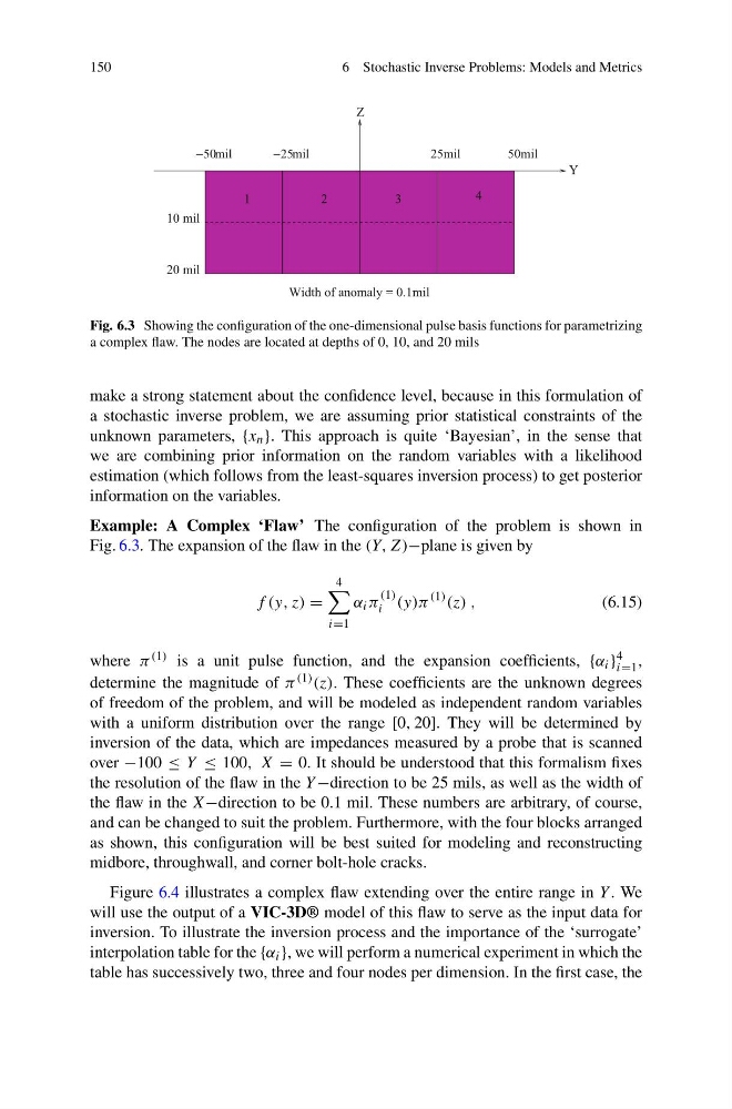
Fig. 6.3 Showing the configuration of the one-dimensional pulse basis functions for parametrizing
a complex flaw. The nodes are located at depths of 0, 10, and 20 mils
make a strong statement about the confidence level, because in this formulation of
a stochastic inverse problem, we are assuming prior statistical constraints of the
unknown parameters, {x n }. This approach is quite ‘Bayesian’, in the sense that
we are combining prior information on the random variables with a likelihood
estimation (which follows from the least-squares inversion process) to get posterior
information on the variables.
Example: A Complex ‘Flaw’ The configuration of the problem is shown in
Fig. 6.3. The expansion of the flaw in the (Y, Z)−plane is given by
f (y, z) =
4
i=1
α i π
(1)
i (y)π
(1) (z) ,
(6.15)
where π (1) is a unit pulse function, and the expansion coefficients, {α i } 4
i=1 ,
determine the magnitude of π (1) (z). These coefficients are the unknown degrees
of freedom of the problem, and will be modeled as independent random variables
with a uniform distribution over the range [0, 20]. They will be determined by
inversion of the data, which are impedances measured by a probe that is scanned
over −100 ≤ Y ≤ 100, X = 0. It should be understood that this formalism fixes
the resolution of the flaw in the Y −direction to be 25 mils, as well as the width of
the flaw in the X−direction to be 0.1 mil. These numbers are arbitrary, of course,
and can be changed to suit the problem. Furthermore, with the four blocks arranged
as shown, this configuration will be best suited for modeling and reconstructing
midbore, throughwall, and corner bolt-hole cracks.
Figure 6.4 illustrates a complex flaw extending over the entire range in Y . We
will use the output of a VIC-3D® model of this flaw to serve as the input data for
inversion. To illustrate the inversion process and the importance of the ‘surrogate’
interpolation table for the {α i }, we will perform a numerical experiment in which the
table has successively two, three and four nodes per dimension. In the first case, the
6 Stochastic Inverse Problems: Models and Metrics
1
4
2
3
Y
Z
20 mil
−25
25
50
Width of anomaly = 0.1mil
mil
mil
−50
10 mil
mil
mil
Fig. 6.3 Showing the configuration of the one-dimensional pulse basis functions for parametrizing
a complex flaw. The nodes are located at depths of 0, 10, and 20 mils
make a strong statement about the confidence level, because in this formulation of
a stochastic inverse problem, we are assuming prior statistical constraints of the
unknown parameters, {x n }. This approach is quite ‘Bayesian’, in the sense that
we are combining prior information on the random variables with a likelihood
estimation (which follows from the least-squares inversion process) to get posterior
information on the variables.
Example: A Complex ‘Flaw’ The configuration of the problem is shown in
Fig. 6.3. The expansion of the flaw in the (Y, Z)−plane is given by
f (y, z) =
4
i=1
α i π
(1)
i (y)π
(1) (z) ,
(6.15)
where π (1) is a unit pulse function, and the expansion coefficients, {α i } 4
i=1 ,
determine the magnitude of π (1) (z). These coefficients are the unknown degrees
of freedom of the problem, and will be modeled as independent random variables
with a uniform distribution over the range [0, 20]. They will be determined by
inversion of the data, which are impedances measured by a probe that is scanned
over −100 ≤ Y ≤ 100, X = 0. It should be understood that this formalism fixes
the resolution of the flaw in the Y −direction to be 25 mils, as well as the width of
the flaw in the X−direction to be 0.1 mil. These numbers are arbitrary, of course,
and can be changed to suit the problem. Furthermore, with the four blocks arranged
as shown, this configuration will be best suited for modeling and reconstructing
midbore, throughwall, and corner bolt-hole cracks.
Figure 6.4 illustrates a complex flaw extending over the entire range in Y . We
will use the output of a VIC-3D® model of this flaw to serve as the input data for
inversion. To illustrate the inversion process and the importance of the ‘surrogate’
interpolation table for the {α i }, we will perform a numerical experiment in which the
table has successively two, three and four nodes per dimension. In the first case, the