

6.4 Summary
155
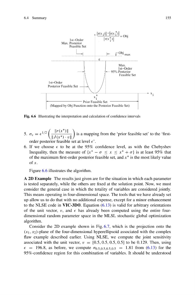
Fig. 6.6 Illustrating the interpretation and calculation of confidence intervals
5. σ v = 1/2
r(x ∗ )
J (x ∗ ) · v
is a mapping from the ‘prior feasible set’ to the ‘firstorder posterior feasible set at level ’.
6. If we choose to be at the 95% confidence level, as with the Chebyshev
Inequality, then the measure of {x ∗ − σ ≤ x ≤ x ∗ + σ } is at least 95% that
of the maximum first-order posterior feasible set, and x ∗ is the most likely value
of x.
Figure 6.6 illustrates the algorithm.
A 2D Example The results just given are for the situation in which each parameter
is tested separately, while the others are fixed at the solution point. Now, we must
consider the general case in which the totality of variables are considered jointly.
This means operating in four-dimensional space. The tools that we have already set
up allow us to do that with no additional expense, except for a minor enhancement
to the NLSE code in VIC-3D®. Equation (6.13) is valid for arbitrary orientations
of the unit vector, v, and has already been computed using the entire fourdimensional random parameter space in the MLSL stochastic global optimization
algorithm.
Consider the 2D example shown in Fig. 6.7, which is the projection onto the
(x 1 , x 2 )-plane of the four-dimensional hyperellipsoid associated with the complex
flaw example described earlier. Using NLSE, we compute the joint sensitivity
associated with the unit vector, v = [0.5, 0.5, 0.5, 0.5] to be 0.129. Then, using
= 196.8, as before, we compute σ 0.5,0.5,0.5,0.5 = 1.81 from (6.13) for the
95%-confidence region for this combination of variables. It should be understood
155
Fig. 6.6 Illustrating the interpretation and calculation of confidence intervals
5. σ v = 1/2
r(x ∗ )
J (x ∗ ) · v
is a mapping from the ‘prior feasible set’ to the ‘firstorder posterior feasible set at level ’.
6. If we choose to be at the 95% confidence level, as with the Chebyshev
Inequality, then the measure of {x ∗ − σ ≤ x ≤ x ∗ + σ } is at least 95% that
of the maximum first-order posterior feasible set, and x ∗ is the most likely value
of x.
Figure 6.6 illustrates the algorithm.
A 2D Example The results just given are for the situation in which each parameter
is tested separately, while the others are fixed at the solution point. Now, we must
consider the general case in which the totality of variables are considered jointly.
This means operating in four-dimensional space. The tools that we have already set
up allow us to do that with no additional expense, except for a minor enhancement
to the NLSE code in VIC-3D®. Equation (6.13) is valid for arbitrary orientations
of the unit vector, v, and has already been computed using the entire fourdimensional random parameter space in the MLSL stochastic global optimization
algorithm.
Consider the 2D example shown in Fig. 6.7, which is the projection onto the
(x 1 , x 2 )-plane of the four-dimensional hyperellipsoid associated with the complex
flaw example described earlier. Using NLSE, we compute the joint sensitivity
associated with the unit vector, v = [0.5, 0.5, 0.5, 0.5] to be 0.129. Then, using
= 196.8, as before, we compute σ 0.5,0.5,0.5,0.5 = 1.81 from (6.13) for the
95%-confidence region for this combination of variables. It should be understood