

148
6 Stochastic Inverse Problems: Models and Metrics
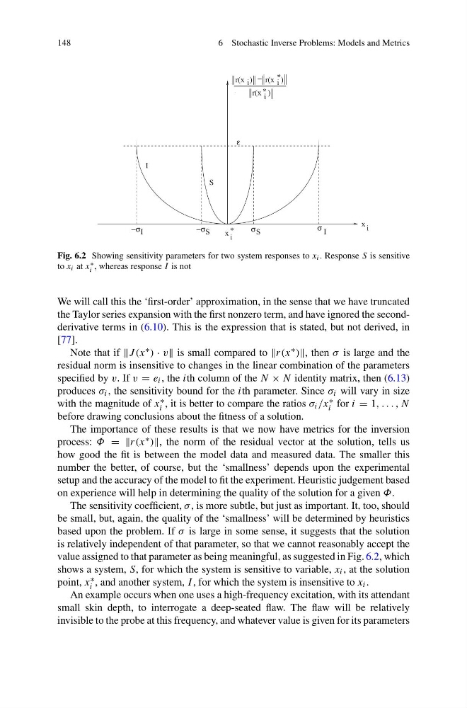
Fig. 6.2 Showing sensitivity parameters for two system responses to x i . Response S is sensitive
to x i at x ∗
i , whereas response I is not
We will call this the ‘first-order’ approximation, in the sense that we have truncated
the Taylor series expansion with the first nonzero term, and have ignored the secondderivative terms in (6.10). This is the expression that is stated, but not derived, in
[77].
Note that if J (x ∗ ) · v is small compared to r(x ∗ ), then σ is large and the
residual norm is insensitive to changes in the linear combination of the parameters
specified by v. If v = e i , the ith column of the N × N identity matrix, then (6.13)
produces σ i , the sensitivity bound for the ith parameter. Since σ i will vary in size
with the magnitude of x ∗
i , it is better to compare the ratios σ i /x ∗
i for i = 1, . . . , N
before drawing conclusions about the fitness of a solution.
The importance of these results is that we now have metrics for the inversion
process: Φ = =r(x ∗ ), the norm of the residual vector at the solution, tells us
how good the fit is between the model data and measured data. The smaller this
number the better, of course, but the ‘smallness’ depends upon the experimental
setup and the accuracy of the model to fit the experiment. Heuristic judgement based
on experience will help in determining the quality of the solution for a given Φ.
The sensitivity coefficient, σ , is more subtle, but just as important. It, too, should
be small, but, again, the quality of the ‘smallness’ will be determined by heuristics
based upon the problem. If σ is large in some sense, it suggests that the solution
is relatively independent of that parameter, so that we cannot reasonably accept the
value assigned to that parameter as being meaningful, as suggested in Fig. 6.2, which
shows a system, S, for which the system is sensitive to variable, x i , at the solution
point, x ∗
i , and another system, I , for which the system is insensitive to x i .
An example occurs when one uses a high-frequency excitation, with its attendant
small skin depth, to interrogate a deep-seated flaw. The flaw will be relatively
invisible to the probe at this frequency, and whatever value is given for its parameters
6 Stochastic Inverse Problems: Models and Metrics
Fig. 6.2 Showing sensitivity parameters for two system responses to x i . Response S is sensitive
to x i at x ∗
i , whereas response I is not
We will call this the ‘first-order’ approximation, in the sense that we have truncated
the Taylor series expansion with the first nonzero term, and have ignored the secondderivative terms in (6.10). This is the expression that is stated, but not derived, in
[77].
Note that if J (x ∗ ) · v is small compared to r(x ∗ ), then σ is large and the
residual norm is insensitive to changes in the linear combination of the parameters
specified by v. If v = e i , the ith column of the N × N identity matrix, then (6.13)
produces σ i , the sensitivity bound for the ith parameter. Since σ i will vary in size
with the magnitude of x ∗
i , it is better to compare the ratios σ i /x ∗
i for i = 1, . . . , N
before drawing conclusions about the fitness of a solution.
The importance of these results is that we now have metrics for the inversion
process: Φ = =r(x ∗ ), the norm of the residual vector at the solution, tells us
how good the fit is between the model data and measured data. The smaller this
number the better, of course, but the ‘smallness’ depends upon the experimental
setup and the accuracy of the model to fit the experiment. Heuristic judgement based
on experience will help in determining the quality of the solution for a given Φ.
The sensitivity coefficient, σ , is more subtle, but just as important. It, too, should
be small, but, again, the quality of the ‘smallness’ will be determined by heuristics
based upon the problem. If σ is large in some sense, it suggests that the solution
is relatively independent of that parameter, so that we cannot reasonably accept the
value assigned to that parameter as being meaningful, as suggested in Fig. 6.2, which
shows a system, S, for which the system is sensitive to variable, x i , at the solution
point, x ∗
i , and another system, I , for which the system is insensitive to x i .
An example occurs when one uses a high-frequency excitation, with its attendant
small skin depth, to interrogate a deep-seated flaw. The flaw will be relatively
invisible to the probe at this frequency, and whatever value is given for its parameters